Interpreting the coefficients of a linear regression

A regression coefficient describes how much the response variable changes for a unit change of a covariate while all other covariates remain constant.

In this notebook, we will deepen this intuition with a hands-on example.

[1]:

import numpy as np
import pandas as pd

import statsmodels.formula.api as smf

import seaborn as sns
import matplotlib.pyplot as plt

[2]:

sns.set_context('poster')

Generate data

We generate synthetic data using a form of structural equation modeling. This way, we can check whether we are able to recover the coefficients.

[3]:

N = 1000

beta_g1 = 1.4
beta_g2 = -0.8

mean_g1 = -2
mean_g2 = 10

[4]:

np.random.seed(42)

X = np.random.normal(size=N * 2)
Y = np.r_[
    beta_g1 * X[: int(len(X) / 2)] + np.random.normal(mean_g1, size=N),
    beta_g2 * X[int(len(X) / 2) :] + np.random.normal(mean_g2, size=N),
]
group = ['$G_1$'] * N + ['$G_2$'] * N

[5]:

df = pd.DataFrame({'X': X, 'Y': Y, 'group': group})

df['group'] = df['group'].astype('category')

df.head()

[5]:

	X	Y	group
0	0.496714	-1.979778	$G_1$
1	-0.138264	-2.338089	$G_1$
2	0.647689	-1.885656	$G_1$
3	1.523030	-0.175720	$G_1$
4	-0.234153	-4.221429	$G_1$

Fit model

The model:

\[Y \sim \beta_0 + \beta_1 \cdot group + \beta_2 \cdot X + \beta_3 \cdot X \cdot group\]

[6]:

mod = smf.ols(formula='Y ~ X * group', data=df)
fit = mod.fit()

Investigate result

Retrieve coefficients

[7]:

res = fit.summary()
res.tables[1]

[7]:

	coef	std err	t	P>\|t\|	[0.025	0.975]
Intercept	-1.9946	0.032	-62.740	0.000	-2.057	-1.932
group[T.$G_2$]	11.9799	0.045	266.149	0.000	11.892	12.068
X	1.4222	0.032	43.793	0.000	1.359	1.486
X:group[T.$G_2$]	-2.2785	0.046	-50.067	0.000	-2.368	-2.189

[8]:

coefs = fit.params
coefs

[8]:

Intercept           -1.994595
group[T.$G_2$]      11.979866
X                    1.422225
X:group[T.$G_2$]    -2.278550
dtype: float64

Understand their meaning

[9]:

fitted_beta_g1 = coefs['X']
fitted_beta_g2 = coefs['X'] + coefs['X:group[T.$G_2$]']

fitted_mean_g1 = coefs['Intercept']
fitted_mean_g2 = coefs['Intercept'] + coefs['group[T.$G_2$]']

[10]:

pd.DataFrame(
    {
        'label': ['beta_g1', 'beta_g2', 'mean_g1', 'mean_g2'],
        'true_value': [beta_g1, beta_g2, mean_g1, mean_g2],
        'fitted_value': [
            fitted_beta_g1,
            fitted_beta_g2,
            fitted_mean_g1,
            fitted_mean_g2,
        ],
    }
)

[10]:

	label	true_value	fitted_value
0	beta_g1	1.4	1.422225
1	beta_g2	-0.8	-0.856325
2	mean_g1	-2.0	-1.994595
3	mean_g2	10.0	9.985271

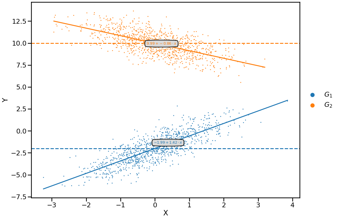
[11]:

def annotate_plot(space, mean, beta, color):
    values = mean + beta * space

    ax.plot(space, values, color=color)
    ax.axhline(mean, ls='dashed', color=color)

    mid = len(space) // 2
    ax.text(
        space[mid],
        values[mid],
        f'${mean:.2f} + {beta:.2f} \cdot x$',
        color=color,
        size=12,
        bbox=dict(boxstyle='round4,pad=.5', fc='0.85'),
        ha='center',
    )

[12]:

plt.figure(figsize=(16, 12))
ax = sns.scatterplot(x='X', y='Y', hue='group', data=df, s=10)

sub = df.loc[df['group'] == '$G_1$', 'X']
annotate_plot(
    np.linspace(sub.min(), sub.max()),
    fitted_mean_g1,
    fitted_beta_g1,
    sns.color_palette()[0],
)

sub = df.loc[df['group'] == '$G_2$', 'X']
annotate_plot(
    np.linspace(sub.min(), sub.max()),
    fitted_mean_g2,
    fitted_beta_g2,
    sns.color_palette()[1],
)

plt.legend(bbox_to_anchor=(1, 0.5), loc='center left', frameon=False)

[12]:

<matplotlib.legend.Legend at 0x10ce91f10>

../_images/stats_ml_LinearRegressionCoefficients_17_1.png