The Art of Life

Nature is remarkably complex and offers a plethora of intricate patterns to those who dare to investigate. These patterns can appear in many forms. Here, we will take a look at how all (sequenced) organisms relate to each other when projecting their high-dimensional genome space down to two dimensions.

import os
import gzip
import json
import shutil
import functools
from pathlib import Path
import multiprocessing as mp
from concurrent.futures import Future, as_completed, ProcessPoolExecutor

import numpy as np
import pandas as pd

import seaborn as sns
import matplotlib.pyplot as plt
from matplotlib.patches import Patch

import requests
from requests_futures.sessions import FuturesSession

import khmer
import metagenompy
from Bio import SeqIO

import umap
import umap.plot

import joblib
from tqdm.auto import tqdm

%matplotlib inline
umap.plot.output_notebook()

Loading BokehJS ...

CPU_COUNT = 10
DATA_DIR = Path("genome_data")

Retrieve Complete Genomes

Before analyzing the genomes, we need to download them. Here, we are going to download (a subset of) all genomes available on RefSeq.

genome_dir = DATA_DIR / "genomes"
genome_dir.mkdir(parents=True, exist_ok=True)

# download assembly info
url = (
    "https://ftp.ncbi.nlm.nih.gov/genomes/ASSEMBLY_REPORTS/assembly_summary_refseq.txt"
)
path_assembly = DATA_DIR / "assembly_information.tsv"

if not path_assembly.exists():
    resp = requests.get(url, stream=True, allow_redirects=True)
    resp.raw.read = functools.partial(resp.raw.read, decode_content=True)
    with tqdm.wrapattr(resp.raw, "read", desc="Download assembly info") as resp_raw:
        with path_assembly.open("wb") as fd:
            shutil.copyfileobj(resp_raw, fd)

# parse assembly info
df_assembly = pd.read_csv(path_assembly, sep="\t", skiprows=1)

# cleaning
df_assembly.rename(
    columns={df_assembly.columns[0]: df_assembly.columns[0].lstrip("#").lstrip()},
    inplace=True,
)

# subsetting
df_assembly = df_assembly[
    (df_assembly["ftp_path"] != "na")
    & (df_assembly["genome_rep"] == "Full")
    & df_assembly["excluded_from_refseq"].isna()
    & (df_assembly["assembly_level"] == "Complete Genome")
]

# summary
print(df_assembly.shape)
df_assembly.head()

(36277, 23)

	assembly_accession	bioproject	biosample	wgs_master	refseq_category	taxid	species_taxid	organism_name	infraspecific_name	isolate	...	genome_rep	seq_rel_date	asm_name	submitter	gbrs_paired_asm	paired_asm_comp	ftp_path	excluded_from_refseq	relation_to_type_material	asm_not_live_date
18	GCF_000002515.2	PRJNA12377	SAMEA3138170	NaN	representative genome	28985	28985	Kluyveromyces lactis	strain=NRRL Y-1140	NaN	...	Full	2004/07/02	ASM251v1	Genolevures Consortium	GCA_000002515.1	different	https://ftp.ncbi.nlm.nih.gov/genomes/all/GCF/0...	NaN	NaN	na
24	GCF_000002725.2	PRJNA15564	SAMEA3138173	NaN	representative genome	347515	5664	Leishmania major strain Friedlin	strain=Friedlin	NaN	...	Full	2011/02/14	ASM272v2	Friedlin Consortium	GCA_000002725.2	identical	https://ftp.ncbi.nlm.nih.gov/genomes/all/GCF/0...	NaN	NaN	na
25	GCF_000002765.5	PRJNA148	SAMN00102897	NaN	representative genome	36329	5833	Plasmodium falciparum 3D7	NaN	3D7	...	Full	2016/04/07	GCA_000002765	Plasmodium falciparum Genome Sequencing Consor...	GCA_000002765.3	different	https://ftp.ncbi.nlm.nih.gov/genomes/all/GCF/0...	NaN	NaN	na
34	GCF_000002985.6	PRJNA158	SAMEA3138177	NaN	reference genome	6239	6239	Caenorhabditis elegans	strain=Bristol N2	NaN	...	Full	2013/02/07	WBcel235	C. elegans Sequencing Consortium	GCA_000002985.3	different	https://ftp.ncbi.nlm.nih.gov/genomes/all/GCF/0...	NaN	NaN	na
65	GCF_000005825.2	PRJNA224116	SAMN02603086	NaN	na	398511	79885	Alkalihalobacillus pseudofirmus OF4	strain=OF4	NaN	...	Full	2010/12/15	ASM582v2	Center for Genomic Sciences, Allegheny-Singer ...	GCA_000005825.2	identical	https://ftp.ncbi.nlm.nih.gov/genomes/all/GCF/0...	NaN	NaN	na

5 rows × 23 columns

def download_genome(row, target_dir, session):
    name = row.ftp_path.rsplit("/", 1)[-1]
    fname = f"{name}_genomic.fna.gz"

    path = target_dir / fname
    meta_path = f"{path}.json"

    url = f"{row.ftp_path}/{fname}"

    if path.exists():
        # print("Using cache for", url)
        future = Future()
        future.set_result("foo")
    else:
        # print("Downloading", url)
        future = session.get(url)

    future.path = path
    future.meta_path = meta_path
    future.accession = row.assembly_accession
    future.taxid = row.taxid

    return future

To speed up the download (which is IO bound), we will distribute this task over multiple threads.

with FuturesSession(max_workers=CPU_COUNT) as session:
    futures = df_assembly.apply(
        download_genome, axis=1, args=(genome_dir, session)
    ).tolist()

    for future in tqdm(
        as_completed(futures), total=len(futures), desc="Download genomes"
    ):
        resp = future.result()

        if isinstance(resp, requests.models.Response):
            with open(future.meta_path, "w") as fd:
                json.dump({"accession": future.accession, "taxid": future.taxid}, fd)

            with open(future.path, mode="wb") as fd:
                fd.write(resp.content)

Compute Genomic Features

We are going to represent DNA sequences by their kmer count profile. In addition, we will compute further statistics, such as, for example, the number of base pairs in each genome.

Helper functions

def load_files(path):
    """Retrieve sequence and metadata for given entry."""
    with gzip.open(path, "rt") as fd:
        record_list = list(SeqIO.parse(fd, "fasta"))

    # aggregate sequences
    seq = ""
    for record in record_list:
        seq += str(record.seq)
    seq = seq.upper()

    # get metadata
    path_meta = f"{path}.json"
    with open(path_meta) as fd:
        metadata = json.load(fd)

    return seq, metadata

def compute_kmer_counts(seq, k=3):
    """
    https://github.com/dib-lab/khmer/blob/master/examples/python-api/exact-counting.py
    """
    # setup counter
    nkmers = 4 ** k
    tablesize = nkmers + 10

    cg = khmer.Countgraph(k, tablesize, 1)
    cg.set_use_bigcount(True)  # increase max count from 255 to 65535

    # count kmers
    cg.consume(seq)

    # return formatted output
    return {cg.reverse_hash(i): cg.get(i) for i in range(nkmers)}

def parse_entry(path):
    """Do all computations for single genome file."""
    assert str(path).endswith("_genomic.fna.gz"), path

    # parse entry
    seq, meta = load_files(path)

    # handle meta information
    meta["genome_size"] = len(seq)

    # count kerms
    kmer_counts = compute_kmer_counts(seq, k=5)

    return meta, kmer_counts

Parse data

As computing these features is CPU bound, we are going to make use of multiprocessing.

kmer_data = {}
metadata = []

with ProcessPoolExecutor(
    max_workers=CPU_COUNT, mp_context=mp.get_context("fork")
) as executor:
    futures = [
        executor.submit(parse_entry, path)
        for path in genome_dir.iterdir()
        if str(path).endswith("_genomic.fna.gz")
    ]

    for future in tqdm(as_completed(futures), total=len(futures), desc="Parse genomes"):
        # compute stuff
        meta, kmer_counts = future.result()

        # keep results
        metadata.append(meta)
        id_ = meta["accession"]

        assert id_ not in kmer_data
        kmer_data[id_] = kmer_counts

Determine taxonomic lineage for each entry

To investigate how different types of organisms relate to each other, we will characterize each organisms by its taxonomic rank.

# list of which ranks to consider
rank_list = ["species", "phylum", "clade", "kingdom", "superkingdom"]

graph = metagenompy.generate_taxonomy_network(auto_download=True)

Parsing names: 100%|██████████| 3532357/3532357 [00:04<00:00, 721381.84it/s]
Parsing nodes: 100%|██████████| 2388279/2388279 [00:21<00:00, 112286.89it/s]

df_meta = pd.DataFrame(metadata).set_index("accession")
df_meta["taxid"] = df_meta["taxid"].astype(str)

df_meta = metagenompy.classify_dataframe(graph, df_meta, rank_list=rank_list)

Classifying: 100%|██████████| 5/5 [00:02<00:00,  2.22it/s]

Save results

df_meta.to_csv(DATA_DIR / "metadata.csv.gz")
df_meta.head()

	taxid	genome_size	species	phylum	clade	kingdom	superkingdom
accession
GCF_002191655.1	29459	3312719	Brucella melitensis	Proteobacteria	<NA>	<NA>	Bacteria
GCF_000852745.1	103881	17266	Potato yellow vein virus	Kitrinoviricota	Riboviria	Orthornavirae	Viruses
GCF_002197575.1	1983777	14964	Avian metaavulavirus 15	Negarnaviricota	Riboviria	Orthornavirae	Viruses
GCF_006384535.1	2588128	59514	Gordonia phage Barb	Uroviricota	Duplodnaviria	Heunggongvirae	Viruses
GCF_000025865.1	547558	2012424	Methanohalophilus mahii	Euryarchaeota	Stenosarchaea group	<NA>	Archaea

df_kmer = pd.DataFrame(kmer_data)
df_kmer.index.name = "kmer"

df_kmer.to_csv(DATA_DIR / "kmer_counts.csv.gz")
df_kmer.head()

	GCF_002191655.1	GCF_000852745.1	GCF_002197575.1	GCF_006384535.1	GCF_000025865.1	GCF_000019085.1	GCF_000800395.1	GCF_000861705.1	GCF_000879055.1	GCF_014127105.1	...	GCF_002448155.1	GCF_016026895.1	GCF_003595175.1	GCF_019192625.1	GCF_018289355.1	GCF_007954485.1	GCF_016403105.1	GCF_011765625.1	GCF_900638255.1	GCF_015571675.1
kmer
AAAAA	7574	120	51	3	15189	37345	2727	63	13	6061	...	1467	16316	4522	22659	36468	42322	12171	33204	7380	23280
AAAAT	7646	160	63	6	11130	27333	1677	44	8	6781	...	1625	11873	2734	17629	28855	34908	11573	28167	6670	18076
AAAAC	7884	72	33	11	7672	12339	2710	47	11	7593	...	3149	13131	4546	16801	19309	22568	10829	20225	8343	17542
AAAAG	9115	77	29	4	10460	24769	3071	40	7	7159	...	2251	6911	3583	12260	26820	23141	8646	18385	4012	12757
AAATA	4774	119	56	11	9577	21599	1022	19	12	3594	...	1328	6824	2166	11850	28194	27460	5007	23131	4916	11996

5 rows × 36277 columns

Data overview

Before analyzing the data in more depth, we check whether reasonable kmer counts have been generated and whether the taxonomic classification worked out.

# did the kmer counting work
max_count_fraction = (df_kmer >= 65535).sum().sum() / (
    df_kmer.shape[0] * df_kmer.shape[1]
)
print(f"{max_count_fraction * 100:.2f}% of kmer counts have reached numeric maximum")

0.08% of kmer counts have reached numeric maximum

# how many NAs are in our taxonomic metadata
df_meta.isna().sum()

taxid               0
genome_size         0
species            27
phylum           2041
clade           15606
kingdom         26965
superkingdom       27
dtype: int64

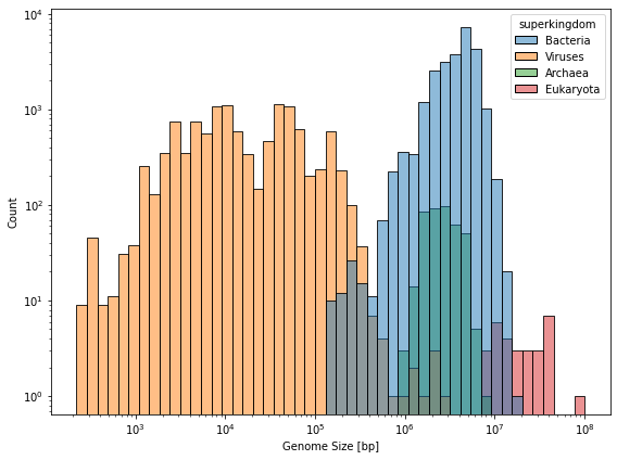
Additionally, we can briefly look at some interesting summary statistics.

fig, ax = plt.subplots(figsize=(8, 6))

sns.histplot(data=df_meta, x="genome_size", hue="superkingdom", log_scale=True, ax=ax)

ax.set_xlabel("Genome Size [bp]")
ax.set_yscale("log")

fig.tight_layout()
fig.savefig(DATA_DIR / "genome_size_hist.pdf")

Kmer statistics

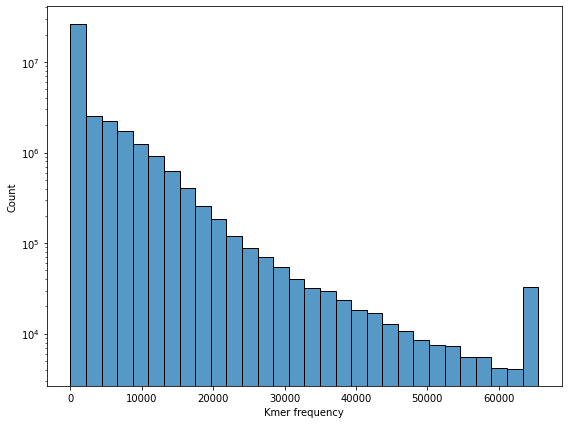
Before reducing the dimensionality of the kmer space, let’s look at a few of its features.

Let’s start by checking the overall kmer count distribution. We can observe a peak at \(0\) as well as a peak at the numeric kmer count maximum of \(65535\).

fig, ax = plt.subplots(figsize=(8, 6))

sns.histplot(data=df_kmer.values.ravel(), bins=30, ax=ax)

ax.set_xlabel("Kmer frequency")
ax.set_yscale("log")

fig.tight_layout()
fig.savefig(DATA_DIR / "kmer_count_hist.pdf")

We then continue by looking at the most/least common kmers averaged over all organisms.

kmer_counts = df_kmer.median(axis=1)
kmer_counts = kmer_counts[kmer_counts > 0]

print("Most common kmers:")
print(kmer_counts.head())
print()
print("Least common (non-zero) kmers:")
print(kmer_counts.tail())

Most common kmers:
kmer
AAAAA    8464.0
AAAAT    6449.0
AAAAC    6518.0
AAAAG    6762.0
AAATA    4391.0
dtype: float64

Least common (non-zero) kmers:
kmer
GCCCC    2177.0
GCCGC    3081.0
GCGCC    2676.0
GGACC    1526.0
GGCCC    1114.0
dtype: float64

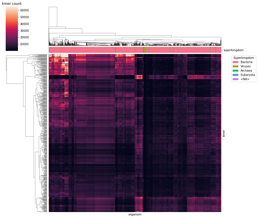
Finally, we can enjoy a clustered heatmap.

%%time

# retain rows with non-zero entries and columns with not-low entries
df_kmer_sub = df_kmer.loc[(df_kmer > 0).any(axis=1), (df_kmer.median(axis=0) > 10)]
df_kmer_sub.columns.rename("organism", inplace=True)

# generate column color map
rank_colors = {
    rank: sns.color_palette("husl", df_meta["superkingdom"].nunique(dropna=False))[i]
    for i, rank in enumerate(df_meta["superkingdom"].unique())
}
rank_cmap = df_meta.loc[df_kmer_sub.columns, "superkingdom"].map(rank_colors)

# create plot
g = sns.clustermap(
    df_kmer_sub,
    col_colors=rank_cmap,
    rasterized=True,
    figsize=(12, 12),
)

g.cax.set_title("kmer count")
g.ax_heatmap.tick_params(bottom=False, labelbottom=False, right=False, labelright=False)

g.ax_heatmap.legend(
    handles=[Patch(facecolor=color, label=name) for name, color in rank_colors.items()],
    title="Superkingdom",
    bbox_to_anchor=(1.05, 1),
    loc="upper left",
)

fig.savefig(DATA_DIR / "kmer_heatmap.pdf", dpi=300)

/cluster/work/bewi/nss/apps/gcc-6.3.0/conda/4.8.3/lib/python3.8/site-packages/seaborn/matrix.py:654: UserWarning: Clustering large matrix with scipy. Installing `fastcluster` may give better performance.
  warnings.warn(msg)

CPU times: user 2min 40s, sys: 6.02 s, total: 2min 46s
Wall time: 2min 47s

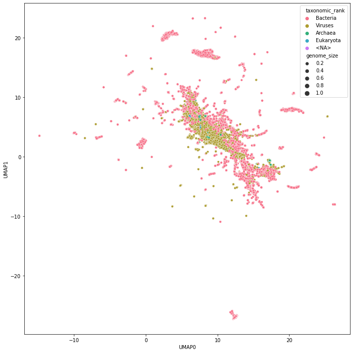
Visualize Projected Genome Space

Finally, we can project the high-dimensional kmer space to two dimensions and explore its topology.

reducer = umap.UMAP(
    metric="cosine",
    random_state=42,
    low_memory=True,
    verbose=True,
    n_neighbors=100,
    n_jobs=min(CPU_COUNT, 8),
)

reducer.fit(df_kmer.T)

UMAP(angular_rp_forest=True, metric='cosine', n_jobs=8, n_neighbors=100, random_state=42, verbose=True)
Wed Jan  5 23:36:01 2022 Construct fuzzy simplicial set
Wed Jan  5 23:36:01 2022 Finding Nearest Neighbors
Wed Jan  5 23:36:01 2022 Building RP forest with 15 trees
Wed Jan  5 23:36:06 2022 NN descent for 15 iterations
         1  /  15
         2  /  15
         3  /  15
        Stopping threshold met -- exiting after 3 iterations
Wed Jan  5 23:37:06 2022 Finished Nearest Neighbor Search
Wed Jan  5 23:37:11 2022 Construct embedding

Wed Jan  5 23:38:22 2022 Finished embedding

UMAP(angular_rp_forest=True, metric='cosine', n_jobs=8, n_neighbors=100, random_state=42, verbose=True)

joblib.dump(reducer, DATA_DIR / "umap_model.joblib")

Wed Jan  5 23:38:27 2022 Worst tree score: 0.96907131
Wed Jan  5 23:38:27 2022 Mean tree score: 0.97277063
Wed Jan  5 23:38:27 2022 Best tree score: 0.97499793
Wed Jan  5 23:38:37 2022 Forward diversification reduced edges from 3627700 to 258377
Wed Jan  5 23:38:40 2022 Reverse diversification reduced edges from 258377 to 257088

/cluster/home/kimja/.local/lib/python3.8/site-packages/scipy/sparse/_index.py:125: SparseEfficiencyWarning: Changing the sparsity structure of a csr_matrix is expensive. lil_matrix is more efficient.
  self._set_arrayXarray(i, j, x)

Wed Jan  5 23:38:42 2022 Degree pruning reduced edges from 297740 to 297717
Wed Jan  5 23:38:42 2022 Resorting data and graph based on tree order
Wed Jan  5 23:38:42 2022 Building and compiling search function

['genome_data/umap_model.joblib']

Static visualization

We can look at a static image…

def format_taxonomy_string(taxonomy, rank_list=["superkingdom", "kingdom"]):
    """Convert classification columns to readable string."""
    return ";".join(str(taxonomy[rank]) for rank in rank_list)

embedding = reducer.transform(df_kmer.T)

df_umap = pd.DataFrame(embedding)
df_umap.columns = ("UMAP0", "UMAP1")
df_umap["accession"] = df_kmer.columns

df_umap["taxonomic_rank"] = df_umap["accession"].apply(
    lambda x: format_taxonomy_string(df_meta.loc[x], rank_list=["superkingdom"])
)

df_umap.set_index("accession", inplace=True)
df_umap["genome_size"] = df_meta["genome_size"]

df_umap.to_csv(DATA_DIR / "umap.csv.gz")
print(df_umap.shape)
df_umap.head()

(36277, 4)

	UMAP0	UMAP1	taxonomic_rank	genome_size
accession
GCF_002191655.1	18.933571	1.356702	Bacteria	3312719
GCF_000852745.1	7.202410	5.276213	Viruses	17266
GCF_002197575.1	7.665549	3.549558	Viruses	14964
GCF_006384535.1	17.502321	-1.682356	Viruses	59514
GCF_000025865.1	8.906975	5.523824	Archaea	2012424

fig, ax = plt.subplots(figsize=(10, 10))

sns.scatterplot(
    data=df_umap,
    x="UMAP0",
    y="UMAP1",
    hue="taxonomic_rank",
    size="genome_size",
    rasterized=True,
    palette=sns.color_palette("husl", df_umap["taxonomic_rank"].nunique()),
    ax=ax,
)

fig.tight_layout()
fig.savefig(DATA_DIR / "umap.pdf", dpi=300)

Interactive visualization

…but also pan and zoom around in an interactive view.

hover_data = df_meta.loc[df_kmer.columns].rename_axis("accession").reset_index()

hover_data["genome_size"] = hover_data["genome_size"].apply(lambda x: f"{x:,} bp")

p = umap.plot.interactive(
    reducer,
    labels=df_umap["taxonomic_rank"].reset_index(drop=True),
    theme="fire",
    hover_data=hover_data,
    point_size=2,
)
umap.plot.show(p)