Analyzing the European Parliament

[1]:

import json

import numpy as np
import pandas as pd

import seaborn as sns
import matplotlib.pyplot as plt
from matplotlib.patches import Patch
import matplotlib.patheffects as PathEffects
from matplotlib.ticker import FuncFormatter, FixedLocator

import bokeh.models as bmo
import bokeh.plotting as bpl
from bokeh.palettes import d3

import prince
import palettable

from tqdm.auto import tqdm

[2]:

sns.set_context('talk')
bpl.output_notebook()

Loading BokehJS ...

Download data

All data is readily available on Parltrack.

[3]:

# %%bash

# wget --no-clobber https://parltrack.org/dumps/ep_votes.json.lz
# lzip -d ep_votes.json.lz

# wget --no-clobber https://parltrack.org/dumps/ep_meps.json.lz
# lzip -d ep_meps.json.lz

Transform JSON to dataframes

To easily work with the data, we transform it from JSON to pandas dataframes.

MEPs

[4]:

fname = 'ep_meps.json'

tmp = []
with open(fname) as fd:
    for line in tqdm(fd.readlines()):
        line = line.lstrip('[,]')
        if len(line) == 0:
            continue

        data = json.loads(line)

        #         if not data['active']:
        #             continue

        tmp.append(
            {
                'UserID': data['UserID'],
                'name': data['Name']['full'],
                'birthday': data['Birth']['date'] if 'Birth' in data else np.nan,
                'active': data['active'],
                'group': data.get('Groups', [{'groupid': np.nan}])[-1][
                    'groupid'
                ],  # assumption: last group is latest one. Is this true?
            }
        )

[5]:

df_meps = pd.DataFrame(tmp)
df_meps['birthday'] = pd.to_datetime(df_meps['birthday'])

df_meps.set_index('UserID', inplace=True)

df_meps['group'].replace(
    {'Group of the European United Left - Nordic Green Left': 'GUE/NGL'}, inplace=True
)  # is there a difference?

df_meps.head()

[5]:

	name	birthday	active	group
UserID
2307	Hubert PIRKER	1948-10-03	False	PPE
111496	María Auxiliadora CORREA ZAMORA	1972-05-24	False	PPE
110987	Gino TREMATERRA	1940-09-03	False	PPE
1965	Jan MULDER	1943-10-03	False	ALDE
39321	Vicente Miguel GARCÉS RAMÓN	1946-11-10	False	S&D

Votes

[6]:

fname = 'ep_votes.json'

tmp = []
tmp_matrix = {}
with open(fname) as fd:
    for line in tqdm(fd.readlines()):
        line = line.lstrip('[,]')
        if len(line) == 0:
            continue

        data = json.loads(line)
        tmp.append(
            {'date': data['ts'], 'voteid': data['voteid'], 'title': data['title']}
        )

        if 'votes' in data:
            tmp_matrix[data['voteid']] = {
                **{
                    mep['mepid']: '+'
                    for mep_list in data['votes']
                    .get('+', {'groups': {'foo': []}})['groups']
                    .values()
                    for mep in mep_list
                    if 'mepid' in mep
                },
                **{
                    mep['mepid']: '-'
                    for mep_list in data['votes']
                    .get('-', {'groups': {'foo': []}})['groups']
                    .values()
                    for mep in mep_list
                    if 'mepid' in mep
                },
                **{
                    mep['mepid']: '0'
                    for mep_list in data['votes']
                    .get('0', {'groups': {'foo': []}})['groups']
                    .values()
                    for mep in mep_list
                    if 'mepid' in mep
                },
            }

[7]:

df_votematrix = pd.DataFrame.from_dict(tmp_matrix, orient='index')

df_votematrix.index.name = 'voteid'
df_votematrix.columns.name = 'mepid'

# df_votematrix.sort_values('voteid', axis=0, inplace=True)
df_votematrix.sort_values('mepid', axis=1, inplace=True)

df_votematrix.head()

[7]:

mepid	1	234	684	729	840	945	966	988	997	1002	...	204416	204418	204419	204420	204421	204443	204449	204733	205452	206158
voteid
7754	NaN	NaN	+	+	NaN	NaN	NaN	NaN	NaN	NaN	...	NaN	NaN	NaN	NaN	NaN	NaN	NaN	NaN	NaN	NaN
7818	-	+	-	-	NaN	-	NaN	NaN	+	-	...	NaN	NaN	NaN	NaN	NaN	NaN	NaN	NaN	NaN	NaN
7759	+	+	+	+	NaN	+	+	NaN	+	NaN	...	NaN	NaN	NaN	NaN	NaN	NaN	NaN	NaN	NaN	NaN
7755	NaN	0	+	NaN	NaN	+	0	NaN	+	+	...	NaN	NaN	NaN	NaN	NaN	NaN	NaN	NaN	NaN	NaN
7760	-	-	-	-	NaN	-	+	NaN	+	-	...	NaN	NaN	NaN	NaN	NaN	NaN	NaN	NaN	NaN	NaN

5 rows × 2329 columns

[8]:

df_votes = pd.DataFrame(tmp)
df_votes['date'] = pd.to_datetime(df_votes['date'])

df_votes.set_index('voteid', inplace=True)

df_votes.tail()

[8]:

	date	title
voteid
116359	2020-07-23 12:49:32	B9-0229/2020 - Am 23
116398	2020-07-23 12:49:32	B9-0229/2020 - § 26/1
116399	2020-07-23 12:49:32	B9-0229/2020 - § 26/2
116360	2020-07-23 12:49:32	B9-0229/2020 - Am 1
116401	2020-07-23 16:52:06	B9-0229/2020 - Résolution

Exploration

We can then look at a few simple statistics.

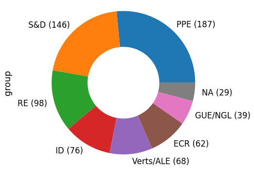
MEP party distribution

How many members (MEPs) does each party of the European parliament have?

[9]:

df_meps['active'].sum()

[9]:

[10]:

group_counts = df_meps.loc[df_meps['active'], 'group'].value_counts()
labels = group_counts.to_frame().apply(lambda x: f'{x.name} ({x.iloc[0]})', axis=1)

ax = group_counts.plot.pie(figsize=(8, 6), labels=labels, wedgeprops=dict(width=0.5))
ax.axis('equal')

[10]:

(-1.1107175100739686,
 1.1005103586792213,
 -1.1057638158926402,
 1.1094386022707399)

../_images/mining_visualization_MEP_Statistics_16_1.png

MEP age distribution

And how old are these members?

[11]:

df_meps['age'] = (pd.Timestamp.today() - df_meps['birthday']) / np.timedelta64(1, 'Y')

[12]:

g = sns.displot(
    data=df_meps[df_meps['active']],
    x='age',
    col='group',
    col_wrap=3,
    height=3,
    aspect=4 / 3,
)

g.set_xlabels('MEP age [years]')

[12]:

<seaborn.axisgrid.FacetGrid at 0x1635ff130>

../_images/mining_visualization_MEP_Statistics_19_1.png

Voting patterns

Let’s now take a look at how these MEPs vote.

[13]:

df_votematrix.head()

[13]:

mepid	1	234	684	729	840	945	966	988	997	1002	...	204416	204418	204419	204420	204421	204443	204449	204733	205452	206158
voteid
7754	NaN	NaN	+	+	NaN	NaN	NaN	NaN	NaN	NaN	...	NaN	NaN	NaN	NaN	NaN	NaN	NaN	NaN	NaN	NaN
7818	-	+	-	-	NaN	-	NaN	NaN	+	-	...	NaN	NaN	NaN	NaN	NaN	NaN	NaN	NaN	NaN	NaN
7759	+	+	+	+	NaN	+	+	NaN	+	NaN	...	NaN	NaN	NaN	NaN	NaN	NaN	NaN	NaN	NaN	NaN
7755	NaN	0	+	NaN	NaN	+	0	NaN	+	+	...	NaN	NaN	NaN	NaN	NaN	NaN	NaN	NaN	NaN	NaN
7760	-	-	-	-	NaN	-	+	NaN	+	-	...	NaN	NaN	NaN	NaN	NaN	NaN	NaN	NaN	NaN	NaN

5 rows × 2329 columns

Who is the most active MEP?

Here we equate “active” with “has voted most often”. This is most likely quite misleading.

[14]:

df_hasvoted = ~df_votematrix[df_meps[df_meps['active']].index].isna()

[15]:

df_hasvoted.sum(axis=0).sort_values(ascending=False).to_frame('vote_count').merge(
    df_meps, how='left', left_index=True, right_index=True
).head(10)

[15]:

	vote_count	name	birthday	active	group	age
mepid
28266	22954	Sophia in 't VELD	1963-09-13	True	RE	57.711345
1913	22703	Evelyne GEBHARDT	1954-01-19	True	S&D	67.359729
2323	22394	Rainer WIELAND	1957-02-19	True	PPE	64.274108
4246	22324	Othmar KARAS	1957-12-24	True	PPE	63.430833
28219	22324	Daniel CASPARY	1976-04-04	True	PPE	45.152566
2341	22269	Michael GAHLER	1960-04-22	True	PPE	61.103612
28224	22164	Markus PIEPER	1963-05-15	True	PPE	58.042632
28298	21992	Iratxe GARCÍA PÉREZ	1974-10-07	True	S&D	46.644725
23821	21912	József SZÁJER	1961-09-07	True	PPE	59.726445
28223	21910	Andreas SCHWAB	1973-04-09	True	PPE	48.139622

Select subset of data

For the subsequent vote clustering, we restrict ourselves to recent votes of active MEPs starting with 2020 (and remove MEPs with no votes at all).

[16]:

df_subset = df_votematrix.loc[
    df_votematrix.index.intersection(df_votes[df_votes['date'] > '2020'].index),
    df_meps[df_meps['active']].index,
].dropna(how='all', axis=1)

print(df_subset.shape)
df_subset.head()

(1808, 703)

[16]:

UserID	96750	4746	23788	96810	96808	4560	38595	1992	125106	4391	...	204413	204334	204331	204346	204449	204400	197780	204733	205452	206158
voteid
111241	0	NaN	NaN	NaN	+	NaN	NaN	NaN	+	NaN	...	NaN	NaN	NaN	NaN	NaN	NaN	NaN	NaN	NaN	NaN
111141	+	NaN	NaN	+	+	+	NaN	NaN	+	NaN	...	NaN	NaN	NaN	NaN	NaN	NaN	NaN	NaN	NaN	NaN
111142	+	NaN	NaN	+	+	+	NaN	+	+	NaN	...	NaN	NaN	NaN	NaN	NaN	NaN	NaN	NaN	NaN	NaN
111143	+	NaN	NaN	+	+	+	NaN	+	+	NaN	...	NaN	NaN	NaN	NaN	NaN	NaN	NaN	NaN	NaN	NaN
111781	-	NaN	NaN	+	-	-	NaN	-	+	NaN	...	NaN	NaN	NaN	NaN	NaN	NaN	NaN	NaN	NaN	NaN

5 rows × 703 columns

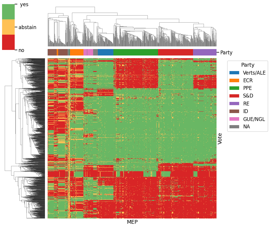
Clustered data overview

Here, we cluster both MEPs and votes as well as highlight each MEP column with their respective party association.

[17]:

# process data to work with clustermap
tmp = df_subset.fillna(0).replace({'+': 1, '0': 0, '-': -1})  # .iloc[:10, :10]
tmp.columns.rename('MEP', inplace=True)
tmp.index.rename('Vote', inplace=True)

# infer party colors
party_colors = {
    party: sns.color_palette('tab10')[i]
    for i, party in enumerate(df_meps.loc[tmp.columns, 'group'].unique())
}
party_cmap = (
    tmp.T.merge(df_meps['group'], how='inner', left_index=True, right_index=True)[
        'group'
    ]
    .map(party_colors)
    .rename('Party')
)

# main plot
g = sns.clustermap(
    tmp,
    col_colors=party_cmap,
    cmap=palettable.tableau.TrafficLight_9.hex_colors[3:6],
    figsize=(12, 12),
)

# plot improvements
g.ax_heatmap.tick_params(bottom=False, labelbottom=False, right=False, labelright=False)


@FuncFormatter
def formatter(x, pos):
    return {-1: 'no', 0: 'abstain', 1: ' yes'}[x]


g.cax.yaxis.set_major_locator(FixedLocator([-1, 0, 1]))
g.cax.yaxis.set_major_formatter(formatter)

# party color legend
g.ax_heatmap.legend(
    handles=[
        Patch(facecolor=color, label=name) for name, color in party_colors.items()
    ],
    title='Party',
    bbox_to_anchor=(1.05, 1),
    loc='upper left',
)

# TODO: improve overall colorbar/legend placement

[17]:

<matplotlib.legend.Legend at 0x155e363a0>

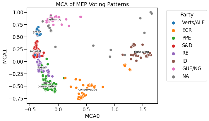
../_images/mining_visualization_MEP_Statistics_28_1.png

Project MEPs based on vote patterns

We will now visualize the landscape of MEPs in two dimensions based on the voting patterns using Multiple Correspondence Analysis.

Apply Multiple Correspondence Analysis (MCA)

[18]:

mca = prince.MCA(n_components=2)
df_mca = mca.fit_transform(df_subset.T)

df_mca.columns = ('MCA0', 'MCA1')
df_mca.index.rename('mepid', inplace=True)
df_mca['group'] = df_meps.loc[df_meps['active'], 'group']

print(df_mca.shape)
df_mca.head()

(703, 3)

[18]:

	MCA0	MCA1	group
mepid
96750	-0.371809	0.631197	Verts/ALE
4746	0.593274	-0.471376	ECR
23788	0.398250	-0.753624	ECR
96810	0.604044	-0.488594	ECR
96808	-0.231881	-0.476251	PPE

Static visualization

[19]:

# obtained from the information box on each party's Wikipedia entry
party_ideology = {
    'Verts/ALE': 'green',
    'ECR': 'conservative',
    'PPE': 'liberal\nconservative',
    'S&D': 'socialist',
    'RE': 'liberal',
    'ID': 'right-wing',
    'GUE/NGL': 'left-wing',
}

[20]:

fig, ax = plt.subplots(figsize=(8, 6))

sns.scatterplot(data=df_mca, x='MCA0', y='MCA1', hue='group', ax=ax)

for party, row in df_mca.groupby('group').mean().iterrows():
    if party == 'NA':
        continue
    ax.text(
        row.MCA0,
        row.MCA1,
        party_ideology.get(party),
        ha='center',
        va='center',
        fontsize=10,
        path_effects=[PathEffects.withStroke(linewidth=3, foreground="w")],
    )

ax.legend(loc='upper left', bbox_to_anchor=(1.05, 1), ncol=1, title='Party')
ax.set_title('MCA of MEP Voting Patterns')

[20]:

Text(0.5, 1.0, 'MCA of MEP Voting Patterns')

../_images/mining_visualization_MEP_Statistics_34_1.png

Interactive visualization

You can zoom and pan the visualization. Hovering over each point (corresponding to a MEP) will display relevant information.

[21]:

# generate data for each tooltip
hover_data = df_meps.loc[df_mca.index]

hover_data['name'] = hover_data['name'].str.title()
hover_data['birthday'] = hover_data['birthday'].apply(
    lambda x: x.strftime("%Y-%m-%d") if not pd.isnull(x) else 'undef'
)
hover_data['age'] = hover_data['age'].apply(
    lambda x: int(x) if not pd.isnull(x) else -1
)

df_data = df_mca.merge(
    hover_data.drop('group', axis=1), left_index=True, right_index=True
)
df_data.head()

[21]:

	MCA0	MCA1	group	name	birthday	active	age
mepid
96750	-0.371809	0.631197	Verts/ALE	François Alfonsi	1953-09-14	True	67
4746	0.593274	-0.471376	ECR	Sergio Berlato	1959-07-27	True	61
23788	0.398250	-0.753624	ECR	Adam Bielan	1974-09-12	True	46
96810	0.604044	-0.488594	ECR	Carlo Fidanza	1976-09-21	True	44
96808	-0.231881	-0.476251	PPE	Pablo Arias Echeverría	1970-06-30	True	50

[22]:

# set up point colors
palette = d3['Category10'][df_data['group'].nunique()]
color_map = bmo.CategoricalColorMapper(
    factors=df_data['group'].unique(), palette=palette
)

[23]:

# create figure
p = bpl.figure(
    tools='hover,pan,reset,wheel_zoom,box_zoom',
    active_scroll='wheel_zoom',
    tooltips=[(col, f'@{col}') for col in hover_data],
    background_fill_color='black',
)

p.scatter(
    x='MCA0',
    y='MCA1',
    color={'field': 'group', 'transform': color_map},
    legend_field='group',
    size=5,
    source=df_data,
)

p.grid.visible = False
p.axis.visible = False

bpl.show(p)