Visualizing Eurostat data

[2]:

import numpy as np
import pandas as pd

import geopandas as gpd

import seaborn as sns
import matplotlib.pyplot as plt
from matplotlib.pyplot import cm

import geoplot as gplt
import geoplot.crs as gcrs

from tqdm.auto import tqdm

from rwrap import eurostat

[3]:

sns.set_context('talk')

Retrieving geographical information

The NUTS classification subdivides each member state into regions at three different levels, covering NUTS 1, 2 and 3 from larger to smaller areas (https://ec.europa.eu/eurostat/web/nuts/background). Eurostat provides this geographical data in various formats (https://ec.europa.eu/eurostat/web/gisco/geodata/reference-data/administrative-units-statistical-units, looks for “NUTS”).

The filename of each dataset follows a specific format: <theme>_<spatialtype>_<resolution>_<year>_<projection>_<subset>.<extension> (check https://ec.europa.eu/eurostat/cache/GISCO/distribution/v2/nuts/nuts-2016-files.html for more information).

To make things easier, we use the eurostat package to retrieve this data automatically.

[5]:

df_geo = eurostat.get_eurostat_geospatial(
    output_class='sf', resolution=60, nuts_level=2, year=2016
)
df_geo.head()

[5]:

	id	CNTR_CODE	NUTS_NAME	LEVL_CODE	FID	NUTS_ID	geometry	geo
0	DE24	DE	Oberfranken	2	DE24	DE24	POLYGON ((11.48157 50.43162, 11.48290 50.40161...	DE24
1	NO03	NO	Sør-Østlandet	2	NO03	NO03	POLYGON ((10.60072 60.13161, 10.57604 60.11572...	NO03
2	HU11	HU	Budapest	2	HU11	HU11	POLYGON ((18.93274 47.57117, 19.02713 47.58717...	HU11
3	HU12	HU	Pest	2	HU12	HU12	POLYGON ((18.96591 47.02896, 18.89943 47.07825...	HU12
4	HU21	HU	Közép-Dunántúl	2	HU21	HU21	POLYGON ((18.68843 47.57707, 18.70448 47.52134...	HU21

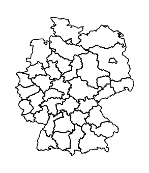
Example

To get a feeling for the data, we can plot the geographical composition of an arbitrary country.

[7]:

ax = gplt.polyplot(df_geo[df_geo['CNTR_CODE'] == 'DE'])
ax.set_aspect(1.4)

../_images/mining_visualization_Eurostat_Visualizations_11_0.png

Retrieving statistical data

Eurostat is a great source for data related to Europe. An overview of the main tables can be found on https://ec.europa.eu/eurostat/web/regions/data/main-tables.

Select datasets

[8]:

eurostat.search_eurostat('age').head()

[8]:

	title	code	type	last update of data	last table structure change	data start	data end	values
1	Manure storage facilities by NUTS 3 regions	aei_fm_ms	dataset	05.02.2019	27.02.2020	2000	2010	None
2	Population on 1 January by age, sex and NUTS 2...	demo_r_d2jan	dataset	13.10.2020	16.06.2020	1990	2019	None
3	Population on 1 January by age group, sex and ...	demo_r_pjangroup	dataset	18.06.2020	14.05.2020	1990	2019	None
4	Population on 1 January by age group, sex and ...	demo_r_pjangrp3	dataset	13.10.2020	14.05.2020	2014	2019	None
5	Population on 1 January by broad age group, se...	demo_r_pjanaggr3	dataset	16.06.2020	16.06.2020	1990	2019	None

[9]:

dataset_list = [
    'tgs00101',  # life expectancy
    'tgs00026',  # exposable income
    'tgs00036',  # primary income
    'tgs00010',  # unemployment rate
    'tgs00112',  # touristic bed number
]

Download and aggregate data

To make the subsequent analysis easier, we download all data at once and store it in a single dataframe. Additionally, we store associated meta data in another dataframe.

[11]:

df_list = []
meta_list = []

for dataset in tqdm(dataset_list):
    # get dataset description
    dataset_name = eurostat.label_eurostat_tables(dataset)[0]
    print(f'Parsing {dataset} ({dataset_name})')

    # retrieve data
    df_data = eurostat.get_eurostat(dataset, time_format='raw')
    df_data = eurostat.label_eurostat(df_data, code=['geo'], fix_duplicated=True)

    # index rows
    common_columns = ['geo_code', 'geo']
    df_data['idx'] = df_data[common_columns].apply(
        lambda row: '_'.join(row.values.astype(str)), axis=1
    )

    # identify meta information
    info_columns = (
        set(df_data.columns)
        - set(common_columns)
        - {'idx', 'time', 'values', 'info', 'info_short'}
    )

    meta_cols = [
        ';'.join(
            f'{k}={row._asdict()[k]}'
            for k in sorted(row._asdict().keys())
            if k != 'Index'
        )
        for row in df_data[info_columns].itertuples()
    ]
    meta_idx, meta_label = pd.factorize(meta_cols)

    df_data['meta'] = [
        f'{dataset}_{time}_{x}' for x, time in zip(meta_idx, df_data['time'])
    ]

    # pivot data
    df_piv = df_data.pivot(index='idx', columns='meta', values='values')

    # store data
    df_list.append(df_piv)

    meta_list.extend(
        [
            {
                'dataset': dataset,
                'name': dataset_name,
                'meta_idx': idx,
                'meta_label': label,
            }
            for idx, label in zip(np.unique(meta_idx), meta_label)
        ]
    )

Parsing tgs00101 (Life expectancy at birth by sex and NUTS 2 region)
Parsing tgs00026 (Disposable income of private households by NUTS 2 regions)
Parsing tgs00036 (Primary income of private households by NUTS 2 regions)
Parsing tgs00010 (Unemployment rate by NUTS 2 regions)
Parsing tgs00112 (Number of establishments and bed-places by NUTS 2 regions)

Each row corresponds to a geographic region, and each column to a certain statistic.

[13]:

df_all = pd.concat(df_list, axis=1)
df_all.head()

[13]:

meta	tgs00101_2007_0	tgs00101_2007_1	tgs00101_2007_2	tgs00101_2008_0	tgs00101_2008_1	tgs00101_2008_2	tgs00101_2009_0	tgs00101_2009_1	tgs00101_2009_2	tgs00101_2010_0	...	tgs00112_2015_0	tgs00112_2015_1	tgs00112_2016_0	tgs00112_2016_1	tgs00112_2017_0	tgs00112_2017_1	tgs00112_2018_0	tgs00112_2018_1	tgs00112_2019_0	tgs00112_2019_1
idx
AT11_Burgenland (AT)	83.3	76.2	79.7	83.4	76.7	80.0	84.2	77.5	80.9	83.9	...	28414.0	436.0	28252.0	427.0	28293.0	427.0	27551.0	418.0	27404.0	412.0
AT12_Niederösterreich	82.7	77.0	79.9	82.8	77.1	80.0	82.7	77.4	80.1	83.3	...	68399.0	1459.0	68714.0	1429.0	67465.0	1434.0	67868.0	1435.0	68246.0	1447.0
AT13_Wien	82.0	76.7	79.5	82.4	77.0	79.9	82.1	76.5	79.4	82.2	...	73901.0	604.0	74771.0	1072.0	75462.0	1212.0	78672.0	1735.0	79245.0	2070.0
AT21_Kärnten	83.6	77.8	80.8	84.1	77.7	81.0	83.7	77.7	80.8	84.0	...	142508.0	2765.0	141191.0	2695.0	140473.0	2717.0	140448.0	2720.0	140165.0	2716.0
AT22_Steiermark	83.6	77.6	80.7	83.7	77.5	80.6	83.5	77.6	80.6	83.9	...	112499.0	2432.0	116262.0	2471.0	118592.0	2471.0	125850.0	2481.0	128815.0	2521.0

5 rows × 120 columns

Extra information for each column is stored in an additional dataframe.

[14]:

df_meta = pd.DataFrame(meta_list)
df_meta.head()

[14]:

	dataset	name	meta_idx	meta_label
0	tgs00101	Life expectancy at birth by sex and NUTS 2 region	0	age=Less than 1 year;sex=Females;unit=Year
1	tgs00101	Life expectancy at birth by sex and NUTS 2 region	1	age=Less than 1 year;sex=Males;unit=Year
2	tgs00101	Life expectancy at birth by sex and NUTS 2 region	2	age=Less than 1 year;sex=Total;unit=Year
3	tgs00026	Disposable income of private households by NUT...	0	direct=Balance;na_item=Disposable income, net;...
4	tgs00036	Primary income of private households by NUTS 2...	0	direct=Balance;na_item=Balance of primary inco...

[15]:

def get_meta(col_name, extended=False):
    dataset, time, idx = col_name.split('_')
    res = df_meta[(df_meta['dataset'] == dataset) & (df_meta['meta_idx'] == int(idx))]
    assert res.shape[0] == 1
    res = res.iloc[0]

    if extended:
        return f'{res["name"]}\n({res["meta_label"]})'
    else:
        return res["name"]

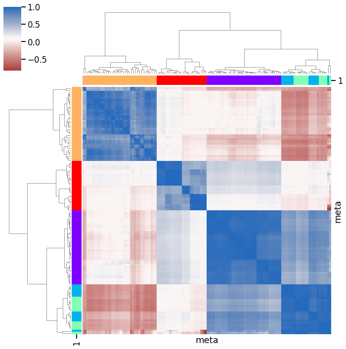
Overview

To get a rough overview of the data, we can plot the clustered correlation matrix.

[16]:

df_corr = df_all.corr()

[17]:

non_nan_datasets = set(df_corr.dropna(axis=0).index) & set(
    df_corr.dropna(axis=1).columns
)
df_corr = df_corr.loc[non_nan_datasets, non_nan_datasets]

[18]:

# assign unique color to each data source
cluster_names = df_all.columns.str.split('_').str[0].unique()
cluser_colors = cm.rainbow(np.linspace(0, 1, len(cluster_names))).tolist()
cluster_map = {n: c for n, c in zip(cluster_names, cluser_colors)}
cluster_colors = pd.DataFrame(
    [(col, cluster_map[col.split('_')[0]]) for col in df_all.columns]
).set_index(0)[1]

[19]:

g = sns.clustermap(
    df_corr,
    xticklabels=False,
    yticklabels=False,
    cmap='vlag_r',
    row_colors=cluster_colors,
    col_colors=cluster_colors,
)

../_images/mining_visualization_Eurostat_Visualizations_30_0.png

Data preparation

In order to combine both geographical and statistical data, we merge the data…

[20]:

df_all['geo_code'] = [idx.split('_')[0] for idx in df_all.index]

[21]:

df_merged = df_geo.merge(df_all, left_on='NUTS_ID', right_on='geo_code')
df_merged.head()

[21]:

	id	CNTR_CODE	NUTS_NAME	LEVL_CODE	FID	NUTS_ID	geometry	geo	tgs00101_2007_0	tgs00101_2007_1	...	tgs00112_2015_1	tgs00112_2016_0	tgs00112_2016_1	tgs00112_2017_0	tgs00112_2017_1	tgs00112_2018_0	tgs00112_2018_1	tgs00112_2019_0	tgs00112_2019_1	geo_code
0	DE24	DE	Oberfranken	2	DE24	DE24	POLYGON ((11.48157 50.43162, 11.48290 50.40161...	DE24	82.2	76.7	...	890.0	40555.0	876.0	40804.0	869.0	40049.0	863.0	41574.0	865.0	DE24
1	NO03	NO	Sør-Østlandet	2	NO03	NO03	POLYGON ((10.60072 60.13161, 10.57604 60.11572...	NO03	82.3	77.7	...	464.0	143032.0	455.0	142724.0	421.0	151654.0	413.0	NaN	NaN	NO03
2	HU11	HU	Budapest	2	HU11	HU11	POLYGON ((18.93274 47.57117, 19.02713 47.58717...	HU11	78.7	72.4	...	342.0	57210.0	359.0	NaN	NaN	56213.0	375.0	58711.0	379.0	HU11
3	HU12	HU	Pest	2	HU12	HU12	POLYGON ((18.96591 47.02896, 18.89943 47.07825...	HU12	77.9	69.8	...	229.0	16348.0	232.0	NaN	NaN	17816.0	248.0	16927.0	240.0	HU12
4	HU21	HU	Közép-Dunántúl	2	HU21	HU21	POLYGON ((18.68843 47.57707, 18.70448 47.52134...	HU21	77.8	69.4	...	610.0	63641.0	625.0	65846.0	651.0	70627.0	685.0	69919.0	692.0	HU21

5 rows × 129 columns

…and dissolve it to reach a resolution which leads to a nice visualization.

[22]:

%%time
df_diss = df_merged.dissolve(by='CNTR_CODE', aggfunc='mean')

CPU times: user 612 ms, sys: 17.3 ms, total: 630 ms
Wall time: 663 ms

[23]:

df_diss.head()

[23]:

	geometry	LEVL_CODE	tgs00101_2007_0	tgs00101_2007_1	tgs00101_2007_2	tgs00101_2008_0	tgs00101_2008_1	tgs00101_2008_2	tgs00101_2009_0	tgs00101_2009_1	...	tgs00112_2015_0	tgs00112_2015_1	tgs00112_2016_0	tgs00112_2016_1	tgs00112_2017_0	tgs00112_2017_1	tgs00112_2018_0	tgs00112_2018_1	tgs00112_2019_0	tgs00112_2019_1
CNTR_CODE
AT	POLYGON ((15.99624 46.83540, 15.98885 46.82563...	2	83.366667	77.611111	80.566667	83.622222	77.977778	80.866667	83.600000	77.844444	...	110385.000000	2257.222222	111271.333333	2291.000000	112577.666667	2320.555556	116181.888889	2388.222222	115356.444444	2439.000000
BE	POLYGON ((6.02490 50.18278, 5.97197 50.17189, ...	2	82.581818	76.909091	79.790909	82.536364	76.627273	79.600000	82.672727	77.190909	...	33499.272727	726.363636	33497.090909	746.363636	33982.000000	779.090909	35438.727273	837.363636	35962.272727	877.363636
BG	POLYGON ((26.56154 41.92627, 26.58121 41.90292...	2	76.466667	69.400000	72.833333	76.850000	69.683333	73.133333	77.183333	70.000000	...	53744.166667	533.666667	54710.666667	555.166667	58120.666667	557.666667	55932.833333	576.333333	56917.666667	610.666667
CH	POLYGON ((9.15938 46.16960, 9.12055 46.13610, ...	2	84.557143	79.614286	82.185714	84.785714	79.942857	82.471429	84.742857	80.014286	...	NaN	NaN	97329.571429	5902.714286	NaN	NaN	94951.857143	5579.571429	NaN	NaN
CY	POLYGON ((33.75237 34.97711, 33.70164 34.97605...	2	82.100000	77.600000	79.800000	82.900000	78.200000	80.600000	83.500000	78.500000	...	85414.000000	788.000000	84239.000000	785.000000	85965.000000	796.000000	87240.000000	802.000000	90188.000000	816.000000

5 rows × 122 columns

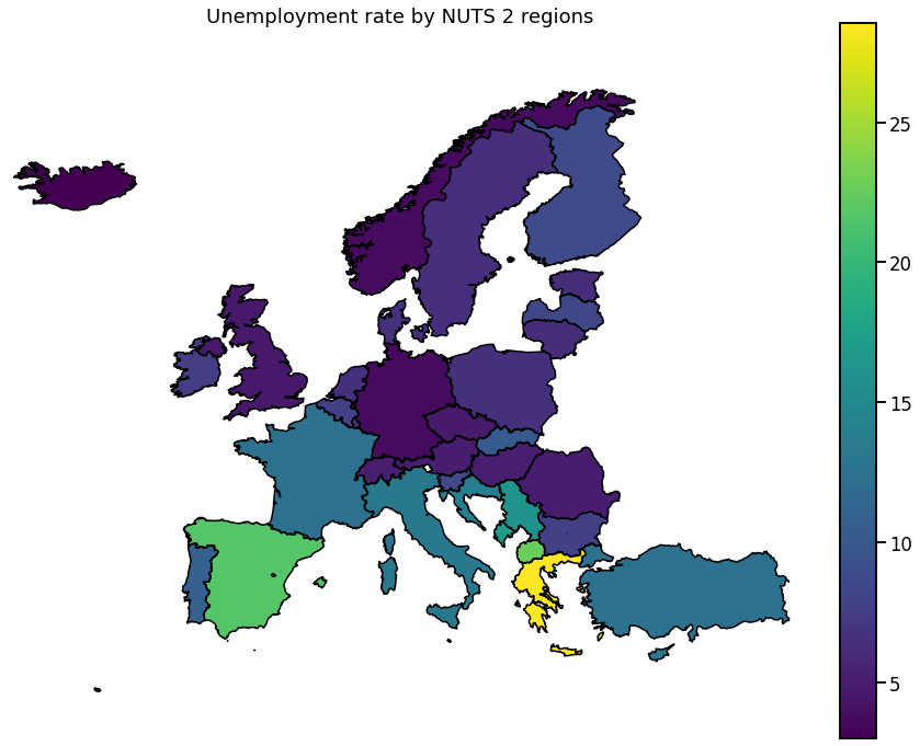
Visualization

We visualize the data using choropleth maps. By doing so, each geographical region is colored according to a statistic of interest.

In the following, we will use a single entry from each downloaded dataset.

[24]:

time = 2016
hue_selection = [
    f'{row.dataset}_{time}_{row.meta_idx}'
    for row in df_meta.groupby('dataset').apply(lambda x: x.sample(n=1)).itertuples()
]
hue_selection

[24]:

['tgs00010_2016_0',
 'tgs00026_2016_0',
 'tgs00036_2016_0',
 'tgs00101_2016_0',
 'tgs00112_2016_0']

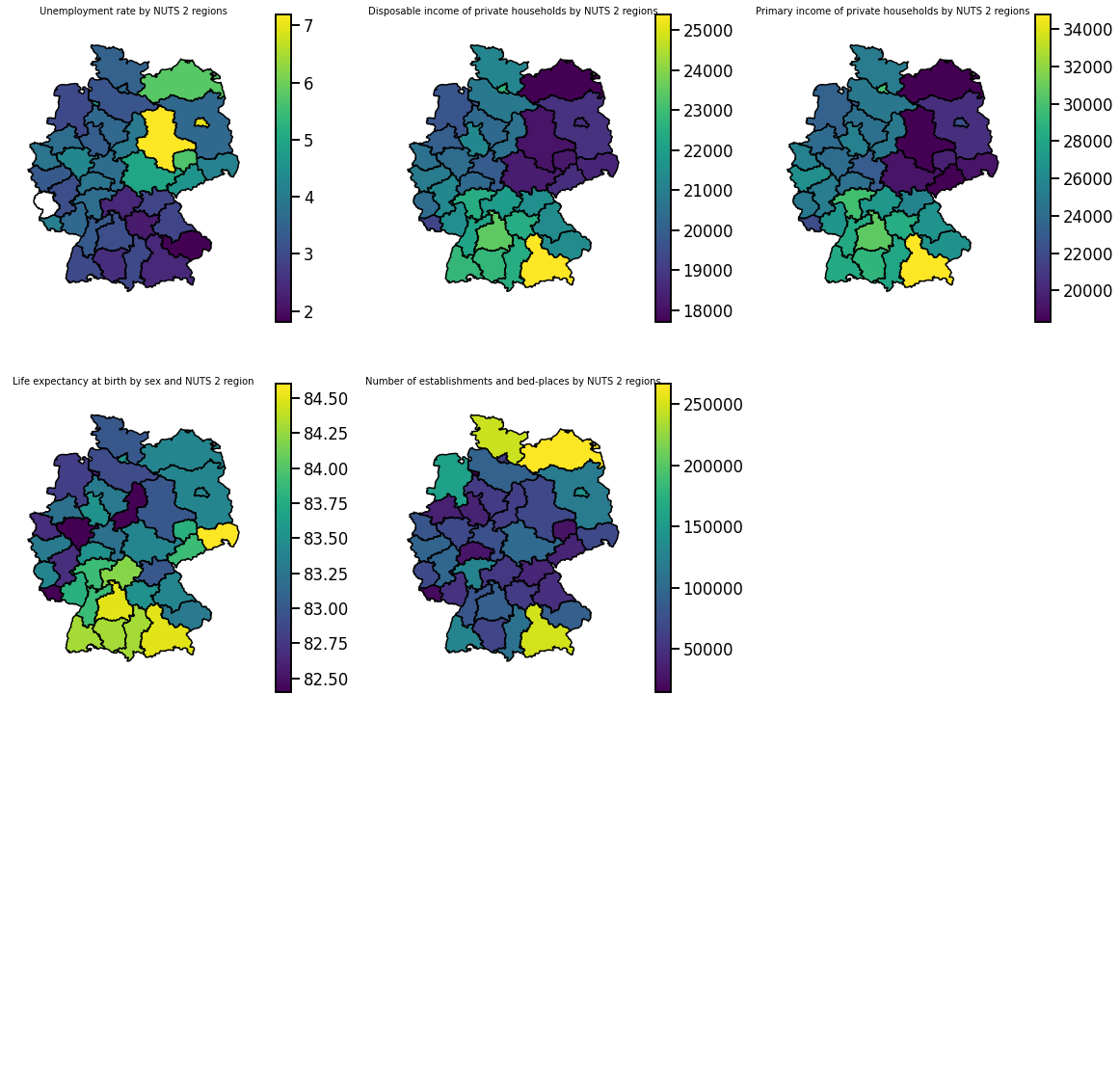
Single country

We can get a precise overview of individual regions within a single country.

[25]:

size = int(np.ceil(np.sqrt(len(hue_selection))))  # size of plot grid

fig, axes = plt.subplots(nrows=size, ncols=size, figsize=(20, 20))
[ax.axis('off') for ax in axes.ravel()]

for hue, ax in zip(hue_selection, axes.ravel()):
    sub = df_merged[(df_merged['CNTR_CODE'] == 'DE')]

    gplt.choropleth(sub, hue=hue, legend=True, ax=ax)
    ax.set_aspect(1.4)
    ax.set_title(get_meta(hue), fontsize=10)

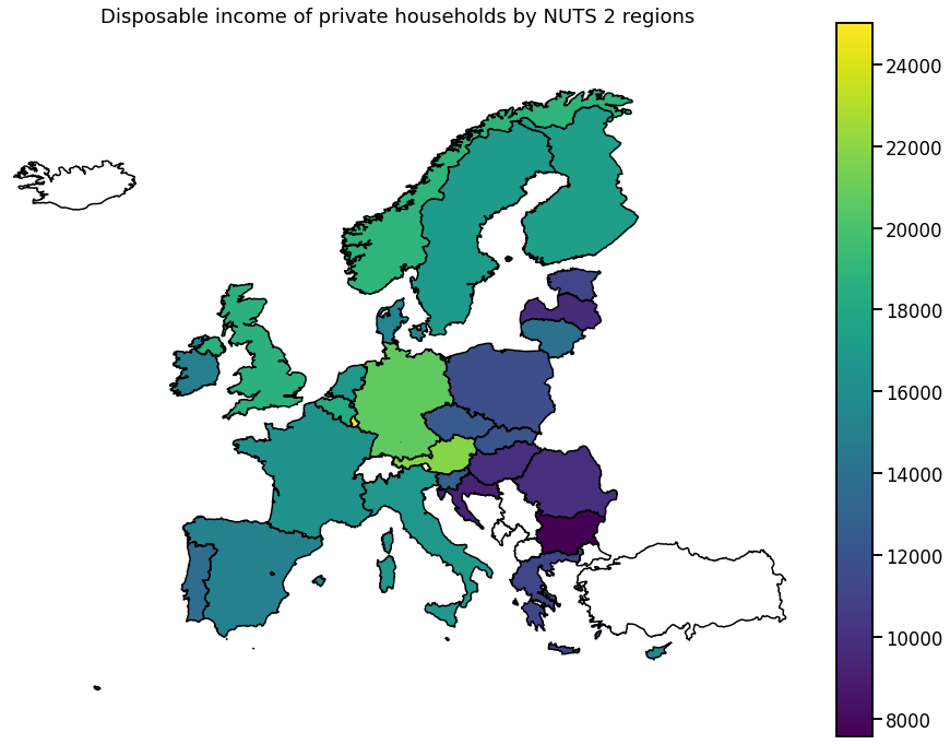
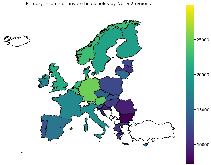
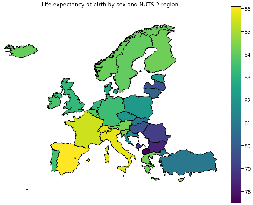
../_images/mining_visualization_Eurostat_Visualizations_40_0.png

Europe

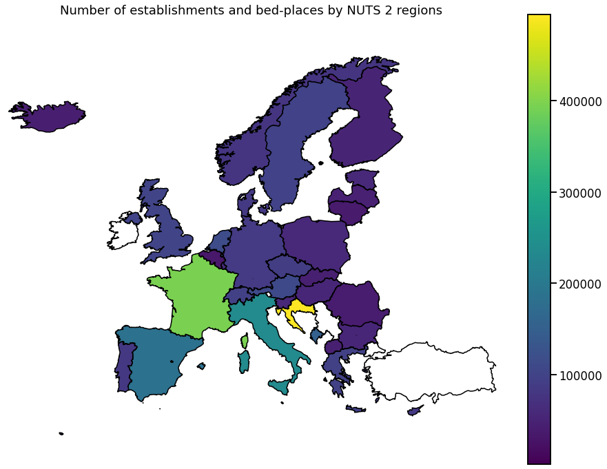
To get a more global picture, we can also plot the aggregated data per country.

[26]:

for hue in hue_selection:
    ax = gplt.choropleth(
        df_diss,
        hue=hue,
        legend=True,  # k=5,
        figsize=(16, 12),
        extent=(
            -25,
            30,
            45,
            75,
        ),  # (min_longitude, min_latitude, max_longitude, max_latitude)
    )
    ax.set_aspect(1.4)
    ax.set_title(get_meta(hue))

../_images/mining_visualization_Eurostat_Visualizations_42_0.png

../_images/mining_visualization_Eurostat_Visualizations_42_1.png

../_images/mining_visualization_Eurostat_Visualizations_42_2.png

../_images/mining_visualization_Eurostat_Visualizations_42_3.png

../_images/mining_visualization_Eurostat_Visualizations_42_4.png