The Python Almanac
The world of Python packages is adventurous and can be confusing at times. Here, I try to aggregate and showcase a diverse set of Python packages which have become useful at some point.
Introduction
Installing Python
Normally you should use your system’s package manager. In case of problems, try pyenv:
$ pyenv versions
$ pyenv install <foo>
$ pyenv global <foo>
This will install the specified Python version to $(pyenv root)/versions.
Installing packages
Python packages can be easily installed from PyPI (Python Package Index):
$ pip install --user <package> (local install does not clash with system packages)
Using --user will install the package only for the current user. This is good if multiple users need different package versions, but can lead to redundant installations.
To install from a git repository, use the following command:
$ pip install --user -U git+https://github.com/<user>/<repository>@<branch>
Package management
While packages can be installed globally or user-specific, it often makes sense to create project-specific virtual environments.
This can be easily accomplished using venv:
$ python -m venv my_venv
$ . venv/bin/activate
$ pip install <package>
Software development
Package Distribution
Use setuptools. poetry handles many otherwise slightly annoying things:
$ poetry init/add/install/run/publish
CI encapsulation: tox.
Keeping track of version numbers can be achieved using bump2version.
Transform between various project file formats using dephell.
Testing
Setup testing using pytest. It has a wide range of useful features, such as fixtures (modularized per-test setup code) and test parametrization (quickly execute the same test for multiple inputs).
[1]:
%%writefile /tmp/tests.py

import os
import pytest


@pytest.fixture(scope='session')
def custom_directory(tmp_path_factory):
    return tmp_path_factory.mktemp('workflow_test')


def test_fixture_execution(custom_directory):
    assert os.path.isdir(custom_directory)


@pytest.mark.parametrize('expression_str,result', [
    ('2+2', 4), ('2*2', 4), ('2**2', 4)
])
def test_expression_evaluation(expression_str, result):
    assert eval(expression_str) == result
Writing /tmp/tests.py
[2]:
!pytest -v /tmp/tests.py
============================= test session starts ==============================
platform darwin -- Python 3.8.6, pytest-6.2.2, py-1.10.0, pluggy-0.13.1 -- /Users/kimja/.pyenv/versions/3.8.6/bin/python3.8
cachedir: .pytest_cache
rootdir: /tmp
plugins: anyio-2.0.2
collected 4 items

../../../../../../../../tmp/tests.py::test_fixture_execution PASSED      [ 25%]
../../../../../../../../tmp/tests.py::test_expression_evaluation[2+2-4] PASSED [ 50%]
../../../../../../../../tmp/tests.py::test_expression_evaluation[2*2-4] PASSED [ 75%]
../../../../../../../../tmp/tests.py::test_expression_evaluation[2**2-4] PASSED [100%]

============================== 4 passed in 0.03s ===============================
Linting/Formatting
Linters and code formatters improve the quality of your Python code by conducting a static analysis and flagging issues.
flake8: Catch various common errors and adhere to PEP8. Supports many plugins.
pylint: Looks for even more sources of code smell.
black: “the uncompromising Python code formatter”.
While there can be a considerable overlap between the tools’ outputs, each offers its own advantages and they can typically be used together.
Profiling
Code profiling tools are a great way of finding parts of your code which can be optimized. They come in various flavors:
line_profiler: which parts of the code require most execution time
memory_profiler: which parts of the code consume the most memory
Consider the following script (note the @profile decorator):
[3]:
%%writefile /tmp/script.py

@profile
def main():
    # takes a long time
    for _ in range(100_000):
        1337**42

    # requires a lot of memory
    arr = [1] * 1_000_000

main()
Writing /tmp/script.py
line_profiler
[4]:
!kernprof -l -v -o /tmp/script.py.lprof /tmp/script.py
Wrote profile results to /tmp/script.py.lprof
Timer unit: 1e-06 s

Total time: 0.13024 s
File: /tmp/script.py
Function: main at line 2

Line #      Hits         Time  Per Hit   % Time  Line Contents
==============================================================
     2                                           @profile
     3                                           def main():
     4                                               # takes a long time
     5    100001      33213.0      0.3     25.5      for _ in range(100_000):
     6    100000      93762.0      0.9     72.0          1337**42
     7
     8                                               # requires a lot of memory
     9         1       3265.0   3265.0      2.5      arr = [1] * 1_000_000
memory_profiler
[5]:
!python3 -m memory_profiler /tmp/script.py
Filename: /tmp/script.py

Line #    Mem usage    Increment  Occurences   Line Contents
============================================================
     2   37.668 MiB   37.668 MiB           1   @profile
     3                                         def main():
     4                                             # takes a long time
     5   37.668 MiB    0.000 MiB      100001       for _ in range(100_000):
     6   37.668 MiB    0.000 MiB      100000           1337**42
     7
     8                                             # requires a lot of memory
     9   45.301 MiB    7.633 MiB           1       arr = [1] * 1_000_000
Debugging
Raw python
ipdb is useful Python commandline debugger. To invoke it, simply put import ipdb; ipdb.set_trace() in your code. Starting with Python 3.7, you can also write breakpoint(). This honors the PYTHONBREAKPOINT environment variable. To automatically start the debugger when an error occurs, run your script with python -m ipdb -c continue <script>.
The debugger supports various commands: * p: print expression * pp: pretty print * n: next line in current function * s: execute current line and stop at next possible location (e.g. in function call) * c: continue execution * unt: execute until we reach greater line * l: list source (l .) * ll: whole source code of current function * b: breakpoint ([ ([filename:]lineno | function) [, condition] ]) * w/bt: print stack trace * u: move up the stack trace * d: move down the
stack trace * h: help * q: quit
C++ extension:
Open two windows: ipython, ldb (gdb)
In [1]: !ps aux | grep -i ipython (lldb) attach –pid 1234 (lldb) continue
(lldb) breakpoint set -f myfile.cpp -l 400
In [2]: run myscript.py
Documentation
sphinx, nbsphinx
Logging
There are various built-in and third-party logging modules available.
[6]:
from loguru import logger
[7]:
logger.debug('Helpful debug message')
logger.error('oh no')
2021-05-01 11:27:35.525 | DEBUG    | __main__:<module>:1 - Helpful debug message
2021-05-01 11:27:35.526 | ERROR    | __main__:<module>:2 - oh no
Data Science
SciPy
SciPy is comprised of various popular Python modules which are for scientific computations.
Numpy can be used for a multitude of things.
[8]:
import numpy as np
[9]:
data = np.random.normal(size=(100, 3))
[10]:
data[:10, :]
[10]:
array([[ 0.12591488, -0.4218942 , -2.12752191],
       [ 1.27252206,  0.22487169, -0.96513306],
       [ 0.42667086, -0.61475518, -0.11270731],
       [ 0.52754573,  0.29209191, -0.03715688],
       [-1.4418503 , -0.45623167, -0.56817326],
       [ 0.53189076,  0.55974594, -0.98371494],
       [ 1.00713651,  0.2159477 ,  0.14132138],
       [ 0.5308628 , -1.82106195, -0.44155486],
       [-1.04296029,  0.16444262, -0.2541122 ],
       [ 0.66799592, -1.62949468,  1.29769595]])
Dataframes
Organizing your data in dataframes using pandas makes nearly everything easier.
[11]:
import pandas as pd
[12]:
df = pd.DataFrame(data, columns=['A', 'B', 'C'])
df['group'] = np.random.choice(['G1', 'G2'], size=df.shape[0])
[13]:
df.head()
[13]:
| A | B | C | group | |
|---|---|---|---|---|
| 0 | 0.125915 | -0.421894 | -2.127522 | G1 |
| 1 | 1.272522 | 0.224872 | -0.965133 | G1 |
| 2 | 0.426671 | -0.614755 | -0.112707 | G1 |
| 3 | 0.527546 | 0.292092 | -0.037157 | G1 |
| 4 | -1.441850 | -0.456232 | -0.568173 | G1 |
Python’s Tidyverse
The philosophy of R’s tidyverse makes working with dataframes a joy. The following packages try to bring these concepts to the world of Python.
siuba as dplyr
siuba implements a grammar of data manipulation inspired by dplyr. It starts by introducing various piping operations to pandas dataframes.
dfply and plydata do (more or less) the same thing.
[14]:
from siuba import group_by, summarize, _
from siuba.data import mtcars
[15]:
(mtcars >> group_by(_.cyl) >> summarize(hp_mean=_.hp.mean()))
[15]:
| cyl | hp_mean | |
|---|---|---|
| 0 | 4 | 82.636364 |
| 1 | 6 | 122.285714 |
| 2 | 8 | 209.214286 |
plotnine as ggplot2
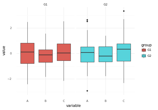
plotnine implements a grammar of graphics and is (in ideology) based on R’s ggplot2.
[16]:
import plotnine
[17]:
# first convert dataframe from wide to long format
df_long = pd.melt(df, id_vars=['group'])
df_long.head()
[17]:
| group | variable | value | |
|---|---|---|---|
| 0 | G1 | A | 0.125915 |
| 1 | G1 | A | 1.272522 |
| 2 | G1 | A | 0.426671 |
| 3 | G1 | A | 0.527546 |
| 4 | G1 | A | -1.441850 |
[18]:
(
    plotnine.ggplot(df_long, plotnine.aes(x='variable', y='value', fill='group'))
    + plotnine.geom_boxplot()
    + plotnine.facet_wrap('~group')
    + plotnine.theme_minimal()
)
[18]:
<ggplot: (334842766)>
pandas-datareader
What fun is data science without data?
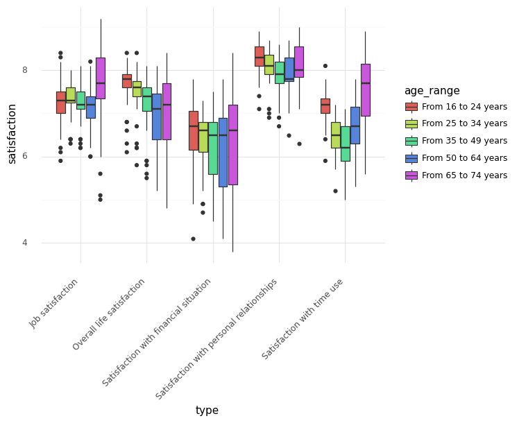
pandas-datareader gives you direct access to a diverse set of data sources.
[19]:
import pandas_datareader as pdr
For example, databases from Eurostat are readily available:
[20]:
# ilc_pw01: Average rating of satisfaction by domain, sex, age and educational attainment level
df_eurostat = pdr.data.DataReader('ilc_pw01', 'eurostat')
df_eurostat.T.head()
[20]:
| TIME_PERIOD | 2018-01-01 | ||||||
|---|---|---|---|---|---|---|---|
| ISCED11 | UNIT | SEX | INDIC_WB | AGE | GEO | FREQ | |
| Less than primary, primary and lower secondary education (levels 0-2) | Rating (0-10) | Females | Satisfaction with accommodation | From 16 to 24 years | Austria | Annual | NaN |
| Belgium | Annual | NaN | |||||
| Bulgaria | Annual | NaN | |||||
| Switzerland | Annual | NaN | |||||
| Cyprus | Annual | NaN |
[21]:
df_eurostat.columns.get_level_values('SEX')
[21]:
Index(['Females', 'Females', 'Females', 'Females', 'Females', 'Females',
       'Females', 'Females', 'Females', 'Females',
       ...
       'Total', 'Total', 'Total', 'Total', 'Total', 'Total', 'Total', 'Total',
       'Total', 'Total'],
      dtype='object', name='SEX', length=58050)
[22]:
df_sub = (
    df_eurostat.T.xs('All ISCED 2011 levels', level='ISCED11')
    .xs('Total', level='SEX')
    .xs('Rating (0-10)', level='UNIT')
    .xs('Annual', level='FREQ')
    .reset_index()
    .drop('GEO', axis=1)
    .rename(
        columns={
            pd.Timestamp('2018-01-01 00:00:00'): 'satisfaction',
            'INDIC_WB': 'type',
            'AGE': 'age_range',
        }
    )
)
df_sub = df_sub[
    df_sub['age_range'].isin(
        [
            'From 16 to 24 years',
            'From 25 to 34 years',
            'From 35 to 49 years',
            'From 50 to 64 years',
            'From 65 to 74 years',
        ]
    )
]
df_sub.dropna().head()
[22]:
| TIME_PERIOD | type | age_range | satisfaction |
|---|---|---|---|
| 774 | Satisfaction with financial situation | From 16 to 24 years | 7.7 |
| 775 | Satisfaction with financial situation | From 16 to 24 years | 7.1 |
| 776 | Satisfaction with financial situation | From 16 to 24 years | 4.1 |
| 777 | Satisfaction with financial situation | From 16 to 24 years | 7.1 |
| 778 | Satisfaction with financial situation | From 16 to 24 years | 6.4 |
[23]:
(
    plotnine.ggplot(
        df_sub.dropna(), plotnine.aes(x='type', y='satisfaction', fill='age_range')
    )
    + plotnine.geom_boxplot()
    + plotnine.theme_minimal()
    + plotnine.theme(axis_text_x=plotnine.element_text(rotation=45, hjust=1))
)
[23]:
<ggplot: (334895665)>
Networkx
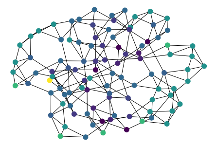
Networkx is a wonderful library for conducting network analysis.
[24]:
import networkx as nx
[25]:
graph = nx.watts_strogatz_graph(100, 4, 0.1)
print(nx.info(graph))
Name:
Type: Graph
Number of nodes: 100
Number of edges: 200
Average degree:   4.0000
[26]:
pos = nx.drawing.nx_agraph.graphviz_layout(graph, prog='neato', args='-Goverlap=scale')
list(pos.items())[:3]
[26]:
[(0, (2800.5, 870.29)), (1, (2479.1, 777.36)), (2, (2464.1, 408.03))]
[27]:
node_clustering = nx.clustering(graph)
list(node_clustering.items())[:3]
[27]:
[(0, 0.5), (1, 0.5), (2, 0.3333333333333333)]
[28]:
nx.draw(
    graph,
    pos,
    node_size=100,
    nodelist=list(node_clustering.keys()),
    node_color=list(node_clustering.values()),
)
Plotting
Matplotlib
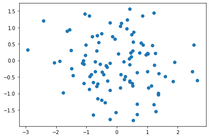
Matplotlib is the de facto standard plotting library for Python.
[29]:
import matplotlib.pyplot as plt
[30]:
fig, ax = plt.subplots()

ax.scatter(data[:, 0], data[:, 1])

fig.tight_layout()
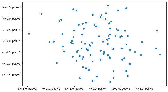
Axis ticks can be formatted in a multitude of different ways. The most versatile way is probably FuncFormatter.
[31]:
from matplotlib.ticker import FuncFormatter
[32]:
@FuncFormatter
def my_formatter(x, pos):
    return f'{x=}, {pos=}'
[33]:
fig, ax = plt.subplots(figsize=(10, 6))

ax.scatter(data[:, 0], data[:, 1])

ax.xaxis.set_major_formatter(my_formatter)
ax.yaxis.set_major_formatter(my_formatter)
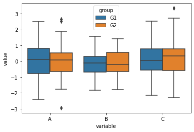
Seaborn
Seaborn makes working with dataframes and creating commonly used plots accessible and comfortable.
[34]:
import seaborn as sns
[35]:
df_long.head()
[35]:
| group | variable | value | |
|---|---|---|---|
| 0 | G1 | A | 0.125915 |
| 1 | G1 | A | 1.272522 |
| 2 | G1 | A | 0.426671 |
| 3 | G1 | A | 0.527546 |
| 4 | G1 | A | -1.441850 |
[36]:
sns.boxplot(data=df_long, x='variable', y='value', hue='group')
[36]:
<AxesSubplot:xlabel='variable', ylabel='value'>
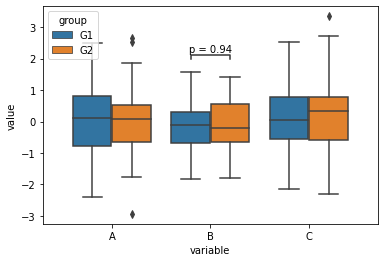
Statannot
Statannot can be used to quickly add markers of significance to comparison plots.
[37]:
import statannot
[38]:
ax = sns.boxplot(
    data=df_long,
    x='variable',
    y='value',
    hue='group',
    order=['A', 'B', 'C'],
    hue_order=['G1', 'G2'],
)

statannot.add_stat_annotation(
    ax,
    plot='barplot',
    data=df_long,
    x='variable',
    y='value',
    hue='group',
    order=['A', 'B', 'C'],
    hue_order=['G1', 'G2'],
    box_pairs=[(('B', 'G1'), ('B', 'G2'))],
    text_format='simple',
    test='Mann-Whitney',
)
B_G1 v.s. B_G2: Mann-Whitney-Wilcoxon test two-sided with Bonferroni correction, P_val=9.415e-01 U_stat=1.207e+03
[38]:
(<AxesSubplot:xlabel='variable', ylabel='value'>,
 [<statannot.StatResult.StatResult at 0x1401d3ca0>])
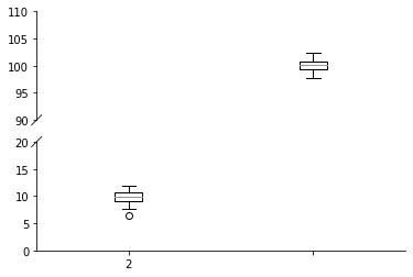
Brokenaxes
Brokenaxes can be used to include outliers in a plot without messing up the axis range. Note that this can be quite misleading.
[39]:
import brokenaxes
[40]:
bax = brokenaxes.brokenaxes(ylims=((0, 20), (90, 110)))
bax.boxplot([np.random.normal(10, size=100), np.random.normal(100, size=100)])
[40]:
[{'whiskers': [<matplotlib.lines.Line2D at 0x14037ba30>,
   <matplotlib.lines.Line2D at 0x14038b3d0>,
   <matplotlib.lines.Line2D at 0x140399850>,
   <matplotlib.lines.Line2D at 0x140399b50>],
  'caps': [<matplotlib.lines.Line2D at 0x14038b730>,
   <matplotlib.lines.Line2D at 0x14038ba90>,
   <matplotlib.lines.Line2D at 0x140399eb0>,
   <matplotlib.lines.Line2D at 0x1403a5250>],
  'boxes': [<matplotlib.lines.Line2D at 0x140385490>,
   <matplotlib.lines.Line2D at 0x1403994f0>],
  'medians': [<matplotlib.lines.Line2D at 0x14038bdf0>,
   <matplotlib.lines.Line2D at 0x1403a55b0>],
  'fliers': [<matplotlib.lines.Line2D at 0x140399190>,
   <matplotlib.lines.Line2D at 0x1403a5910>],
  'means': []},
 {'whiskers': [<matplotlib.lines.Line2D at 0x1403af040>,
   <matplotlib.lines.Line2D at 0x1403af3a0>,
   <matplotlib.lines.Line2D at 0x1403ba6d0>,
   <matplotlib.lines.Line2D at 0x1403baa30>],
  'caps': [<matplotlib.lines.Line2D at 0x1403af5b0>,
   <matplotlib.lines.Line2D at 0x1403af910>,
   <matplotlib.lines.Line2D at 0x1403bad90>,
   <matplotlib.lines.Line2D at 0x1403c7100>],
  'boxes': [<matplotlib.lines.Line2D at 0x1403a5ca0>,
   <matplotlib.lines.Line2D at 0x1403ba370>],
  'medians': [<matplotlib.lines.Line2D at 0x1403afc70>,
   <matplotlib.lines.Line2D at 0x1403c7460>],
  'fliers': [<matplotlib.lines.Line2D at 0x1403affd0>,
   <matplotlib.lines.Line2D at 0x1403c77c0>],
  'means': []}]
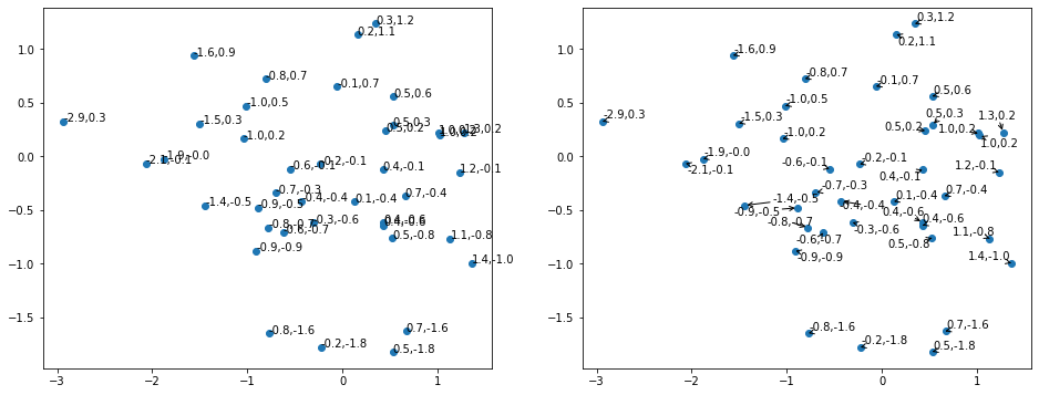
Adjusttext
Adjusttext can help for plots with many labels which potentially overlap.
[41]:
from adjustText import adjust_text
[42]:
data_sub = data[:40, :]
fig, (ax_raw, ax_adj) = plt.subplots(nrows=1, ncols=2, figsize=(16, 6))

ax_raw.scatter(data_sub[:, 0], data_sub[:, 1])
[
    ax_raw.annotate(f'{round(x, 1)},{round(y, 1)}', xy=(x, y))
    for x, y in data_sub[:, [0, 1]]
]

ax_adj.scatter(data_sub[:, 0], data_sub[:, 1])
adjust_text(
    [
        ax_adj.annotate(f'{round(x, 1)},{round(y, 1)}', xy=(x, y))
        for x, y in data_sub[:, [0, 1]]
    ],
    arrowprops=dict(arrowstyle='->'),
)
[42]:
182
Folium
Folium is a Python wrapper of the Leaflet.js library to visualize dynamic maps.
[43]:
import folium
[44]:
folium.Map(
    location=[np.random.uniform(40, 70), np.random.uniform(10, 30)],
    zoom_start=7,
    width=500,
    height=500,
)
[44]:
Ahlive
Creating animated visualizations becomes easy and fun with ahlive.
[45]:
import ahlive as ah
[46]:
adf = ah.DataFrame(pd.DataFrame({'A': [1, 2, 3], 'B': [1, 2, 3]}), xs='A', ys='B')

adf.render()
[########################################] | 100% Completed | 6.5s
[46]:

Color palettes
Choosing the right color palette for your visualization can be tricky. palettable provides many useful ones.
[47]:
import palettable
You can easily display a multitude of colorscales…
[48]:
palettable.tableau.Tableau_10.show_discrete_image()

…and access them in a variety of ways.
[49]:
print(palettable.tableau.Tableau_10.name)
print(palettable.tableau.Tableau_10.type)
print(palettable.tableau.Tableau_10.hex_colors)
print(palettable.tableau.Tableau_10.mpl_colormap)
Tableau_10
qualitative
['#1F77B4', '#FF7F0E', '#2CA02C', '#D62728', '#9467BD', '#8C564B', '#E377C2', '#7F7F7F', '#BCBD22', '#17BECF']
<matplotlib.colors.LinearSegmentedColormap object at 0x1426fcac0>
High performance
When dealing with large amounts of data or many computations, it can make sense to optimize hotspots in C++ or use specialized libraries.
Dask
Dask provides a Panda’s like interface to high-performance dataframes which support out-of-memory processing, cluster distribution, and more. It is particularly useful when the dataframe does not fit in RAM anymore. Common operations operate on chunks of the dataframe and are only executed when explicitly requested.
[50]:
import dask.dataframe as dd
[51]:
df = pd.DataFrame(np.random.normal(size=(1_000_000, 2)), columns=['A', 'B'])
[52]:
ddf = dd.from_pandas(df, npartitions=4)
ddf.head()
[52]:
| A | B | |
|---|---|---|
| 0 | 1.209945 | -0.829657 |
| 1 | -1.041410 | 0.138946 |
| 2 | 0.497872 | 0.628439 |
| 3 | -0.418077 | 0.039312 |
| 4 | -0.353732 | 0.500529 |
[53]:
ddf['A'] + ddf['B']
[53]:
Dask Series Structure:
npartitions=4
0         float64
250000        ...
500000        ...
750000        ...
999999        ...
dtype: float64
Dask Name: add, 16 tasks
[54]:
(ddf['A'] + ddf['B']).compute()
[54]:
0         0.380288
1        -0.902464
2         1.126310
3        -0.378765
4         0.146798
            ...
999995   -1.198871
999996    0.195255
999997    1.707589
999998   -1.505217
999999   -1.828147
Length: 1000000, dtype: float64
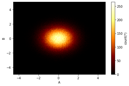
Vaex
Vaex fills a similar niche as dask and makes working with out-of-core dataframe easy. It has a slightly more intuitive interface and offers many cool visualizations right out of the box.
[55]:
import vaex as vx
[56]:
vdf = vx.from_pandas(df)
vdf.head()
[56]:
| # | A | B |
|---|---|---|
| 0 | 1.20994 | -0.829657 |
| 1 | -1.04141 | 0.138946 |
| 2 | 0.497872 | 0.628439 |
| 3 | -0.418077 | 0.0393116 |
| 4 | -0.353732 | 0.500529 |
| 5 | 0.218921 | -0.140769 |
| 6 | 1.44677 | 0.177711 |
| 7 | -0.929196 | -0.306118 |
| 8 | 1.23181 | 1.37377 |
| 9 | -0.354355 | -1.17795 |
[57]:
vdf['A'] + vdf['B']
[57]:
Expression = (A + B)
Length: 1,000,000 dtype: float64 (expression)
---------------------------------------------
     0   0.380288
     1  -0.902464
     2    1.12631
     3  -0.378765
     4   0.146798
       ...
999995   -1.19887
999996   0.195255
999997    1.70759
999998   -1.50522
999999   -1.82815
[58]:
vdf.plot(vdf['A'], vdf['B'])
[58]:
<matplotlib.image.AxesImage at 0x141ea3310>
Joblib
Joblib makes executing functions in parallel very easy and removes boilerplate code.
[59]:
import time
import random

import joblib
[60]:
def heavy_function(i):
    print(f'{i=}')
    time.sleep(random.random())
    return i**i
[61]:
joblib.Parallel(n_jobs=2)([joblib.delayed(heavy_function)(i) for i in range(10)])
[61]:
[1, 1, 4, 27, 256, 3125, 46656, 823543, 16777216, 387420489]
Swifter
Choosing the correct way of parallelizing your computations can be non-trivial. Swifter tries to automatically select the most suitable one.
[62]:
import swifter
[63]:
df_big = pd.DataFrame({'A': np.random.randint(0, 100, size=1_000_000)})
df_big.head()
[63]:
| A | |
|---|---|
| 0 | 29 |
| 1 | 84 |
| 2 | 61 |
| 3 | 63 |
| 4 | 39 |
[64]:
%%timeit
df_big['A'].apply(lambda x: x**2)
526 ms ± 4.48 ms per loop (mean ± std. dev. of 7 runs, 1 loop each)
[65]:
%%timeit
df_big['A'].swifter.apply(lambda x: x**2)
2.84 ms ± 139 µs per loop (mean ± std. dev. of 7 runs, 100 loops each)
Bioinformatics
PyRanges
PyRanges makes working with genomic ranges easy as pie.
[66]:
import pyranges as pr
[67]:
df_exons = pr.data.exons()
df_exons
[67]:
+--------------+-----------+-----------+-------+
| Chromosome   | Start     | End       | +3    |
| (category)   | (int32)   | (int32)   | ...   |
|--------------+-----------+-----------+-------|
| chrX         | 135721701 | 135721963 | ...   |
| chrX         | 135574120 | 135574598 | ...   |
| chrX         | 47868945  | 47869126  | ...   |
| chrX         | 77294333  | 77294480  | ...   |
| ...          | ...       | ...       | ...   |
| chrY         | 15409586  | 15409728  | ...   |
| chrY         | 15478146  | 15478273  | ...   |
| chrY         | 15360258  | 15361762  | ...   |
| chrY         | 15467254  | 15467278  | ...   |
+--------------+-----------+-----------+-------+
Stranded PyRanges object has 1,000 rows and 6 columns from 2 chromosomes.
For printing, the PyRanges was sorted on Chromosome and Strand.
3 hidden columns: Name, Score, Strand
[68]:
df_locus = pr.PyRanges(
    pd.DataFrame({'Chromosome': ['chrX'], 'Start': [1_400_000], 'End': [1_500_000]})
)
df_locus
[68]:
+--------------+-----------+-----------+
| Chromosome   |     Start |       End |
| (category)   |   (int32) |   (int32) |
|--------------+-----------+-----------|
| chrX         |   1400000 |   1500000 |
+--------------+-----------+-----------+
Unstranded PyRanges object has 1 rows and 3 columns from 1 chromosomes.
For printing, the PyRanges was sorted on Chromosome.
[69]:
df_exons.overlap(df_locus).df
[69]:
| Chromosome | Start | End | Name | Score | Strand | |
|---|---|---|---|---|---|---|
| 0 | chrX | 1475113 | 1475229 | NM_001267713_exon_4_0_chrX_1475114_f | 0 | + |
| 1 | chrX | 1419383 | 1419519 | NM_001161531_exon_9_0_chrX_1419384_f | 0 | + |
| 2 | chrX | 1424338 | 1424420 | NM_006140_exon_11_0_chrX_1424339_f | 0 | + |
| 3 | chrX | 1407651 | 1407781 | NM_001161532_exon_3_0_chrX_1407652_f | 0 | + |
| 4 | chrX | 1404670 | 1404813 | NM_172245_exon_3_0_chrX_1404671_f | 0 | + |
| 5 | chrX | 1424338 | 1424420 | NM_001161530_exon_10_0_chrX_1424339_f | 0 | + |
| 6 | chrX | 1414319 | 1414349 | NM_172245_exon_8_0_chrX_1414320_f | 0 | + |
| 7 | chrX | 1407411 | 1407535 | NM_172249_exon_4_0_chrX_1407412_f | 0 | + |
Obonet
Obonet is a library for working with (OBO-formatted) ontologies.
[70]:
import obonet
[71]:
url = 'https://github.com/DiseaseOntology/HumanDiseaseOntology/raw/main/src/ontology/HumanDO.obo'
graph = obonet.read_obo(url)
[72]:
list(graph.nodes(data=True))[0]
[72]:
('DOID:0001816',
 {'name': 'angiosarcoma',
  'alt_id': ['DOID:267', 'DOID:4508'],
  'def': '"A vascular cancer that derives_from the cells that line the walls of blood vessels or lymphatic vessels." [url:http\\://en.wikipedia.org/wiki/Hemangiosarcoma, url:https\\://en.wikipedia.org/wiki/Angiosarcoma, url:https\\://ncit.nci.nih.gov/ncitbrowser/ConceptReport.jsp?dictionary=NCI_Thesaurus&ns=ncit&code=C3088, url:https\\://www.ncbi.nlm.nih.gov/pubmed/23327728]',
  'subset': ['DO_cancer_slim', 'NCIthesaurus'],
  'synonym': ['"hemangiosarcoma" EXACT []'],
  'xref': ['ICDO:9120/3',
   'MESH:D006394',
   'NCI:C3088',
   'NCI:C9275',
   'SNOMEDCT_US_2020_09_01:39000009',
   'UMLS_CUI:C0018923',
   'UMLS_CUI:C0854893'],
  'is_a': ['DOID:175']})
Statistics/Machine Learning
Statsmodels
Statsmodels helps with statistical modelling.
[73]:
import statsmodels.formula.api as smf
[74]:
df_data = pd.DataFrame({'X': np.random.normal(size=100)})

df_data['Y'] = 1.3 * df_data['X'] + 4.2

df_data.head()
[74]:
| X | Y | |
|---|---|---|
| 0 | 0.927521 | 5.405777 |
| 1 | 2.110368 | 6.943479 |
| 2 | 1.517580 | 6.172854 |
| 3 | -0.069583 | 4.109542 |
| 4 | -0.644390 | 3.362293 |
[75]:
mod = smf.ols('Y ~ X', data=df_data)
res = mod.fit()
[76]:
res.params
[76]:
Intercept    4.2
X            1.3
dtype: float64
[77]:
res.summary().tables[1]
[77]:
| coef | std err | t | P>|t| | [0.025 | 0.975] | |
|---|---|---|---|---|---|---|
| Intercept | 4.2000 | 2.03e-16 | 2.07e+16 | 0.000 | 4.200 | 4.200 |
| X | 1.3000 | 1.93e-16 | 6.73e+15 | 0.000 | 1.300 | 1.300 |
Pingouin
Pingouin provides additional statistical methods.
[78]:
import pingouin as pg
[79]:
pg.normality(np.random.normal(size=100))
/Users/kimja/.pyenv/versions/3.8.6/lib/python3.8/site-packages/outdated/utils.py:14: OutdatedPackageWarning: The package outdated is out of date. Your version is 0.2.0, the latest is 0.2.1.
Set the environment variable OUTDATED_IGNORE=1 to disable these warnings.
/Users/kimja/.pyenv/versions/3.8.6/lib/python3.8/site-packages/outdated/utils.py:14: OutdatedPackageWarning: The package pingouin is out of date. Your version is 0.3.9, the latest is 0.3.11.
Set the environment variable OUTDATED_IGNORE=1 to disable these warnings.
[79]:
| W | pval | normal | |
|---|---|---|---|
| 0 | 0.985349 | 0.336443 | True |
[80]:
pg.normality(np.random.uniform(size=100))
[80]:
| W | pval | normal | |
|---|---|---|---|
| 0 | 0.946713 | 0.000507 | False |
Scitkit-learn
Scikit-learn facilitates machine learning in Python.
[81]:
from sklearn import svm
from sklearn import datasets
from sklearn.model_selection import train_test_split
[82]:
X, y = datasets.load_iris(return_X_y=True)
X.shape, y.shape
[82]:
((150, 4), (150,))
[83]:
X_train, X_test, y_train, y_test = train_test_split(X, y, test_size=0.4, random_state=0)
[84]:
clf = svm.SVC(kernel='linear', C=1).fit(X_train, y_train)
clf.score(X_test, y_test)
[84]:
0.9666666666666667
Scikit-learn offers various plugins which deal with common issues encountered while modeling.
Imbalanced-learn provides various re-sampling techniques when the dataset has annoying class imbalances.
[85]:
import collections

from imblearn.over_sampling import RandomOverSampler
[86]:
ros = RandomOverSampler(random_state=0)
[87]:
X_sub, y_sub = X[:60, :], y[:60]
X_resampled, y_resampled = ros.fit_resample(X_sub, y_sub)
[88]:
print('sub:', sorted(collections.Counter(y_sub).items()))
print('resampled:', sorted(collections.Counter(y_resampled).items()))
sub: [(0, 50), (1, 10)]
resampled: [(0, 50), (1, 50)]
Category_encoders helps with converting categorical variables to numerical ones.
[89]:
import category_encoders
[90]:
tmp = np.random.choice(['A', 'B'], size=10)
df_cat = pd.DataFrame({'original_class': tmp, 'feature01': tmp})
df_cat.head()
[90]:
| original_class | feature01 | |
|---|---|---|
| 0 | A | A |
| 1 | B | B |
| 2 | A | A |
| 3 | A | A |
| 4 | B | B |
[91]:
category_encoders.OneHotEncoder(cols=['feature01']).fit_transform(df_cat)
[91]:
| original_class | feature01_1 | feature01_2 | |
|---|---|---|---|
| 0 | A | 1 | 0 |
| 1 | B | 0 | 1 |
| 2 | A | 1 | 0 |
| 3 | A | 1 | 0 |
| 4 | B | 0 | 1 |
| 5 | B | 0 | 1 |
| 6 | B | 0 | 1 |
| 7 | B | 0 | 1 |
| 8 | B | 0 | 1 |
| 9 | B | 0 | 1 |
Yellowbrick makes a multitude of visual diagnostic tools readily accessible.
[92]:
from yellowbrick.classifier import ROCAUC
[93]:
clf.fit(X, y)
[93]:
SVC(C=1, kernel='linear')
[94]:
visualizer = ROCAUC(clf)
# visualizer.score(X, y)  # TODO: uncomment once scikit-learn is fixed
visualizer.show()
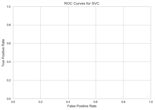
[94]:
<AxesSubplot:title={'center':'ROC Curves for SVC'}, xlabel='False Positive Rate', ylabel='True Positive Rate'>
Language Bindings
Pybind11
Pybind11 makes writing bindings between Python and C++ enjoyable. In combination with cppimport some might even call it fun. It is possible to implement custom typecasters to support bindings for arbitrary objects.
[95]:
%%writefile cpp_source.cpp

#include <pybind11/pybind11.h>

namespace py = pybind11;


int square(int x) {
    return x * x;
}

PYBIND11_MODULE(cpp_source, m) {
    m.def(
        "square", &square,
        py::arg("x") = 1
    );
}

/*
<%
setup_pybind11(cfg)
cfg['compiler_args'] = ['-std=c++11']
%>
*/
Overwriting cpp_source.cpp
[96]:
import cppimport
[97]:
cpp_source = cppimport.imp('cpp_source')
[98]:
cpp_source.square(5)
[98]:
25
Jupyter
Nbstripout
Commiting Jupyter notebooks to CVS (e.g. git) can be annoying due to non-code properties being saved. Nbstripout strips all of those away and can be run automatically for each committed notebook by executing nbstripout --install once.
Miscellaneous
humanize
humanize allows to format numbers with the goal of making them more human-readable.
[99]:
import datetime

import humanize
This is, of course, highly context-dependent:
[100]:
big_number = 4578934

print('Actual number:', big_number)
print('Readable number:', humanize.intword(big_number))
print('Time difference:', humanize.precisedelta(datetime.timedelta(seconds=big_number)))
print('File size:', humanize.naturalsize(big_number))
Actual number: 4578934
Readable number: 4.6 million
Time difference: 1 month, 21 days, 23 hours, 55 minutes and 34 seconds
File size: 4.6 MB
rich
Making sure that terminal applications have nicely formatted output makes using them a much better experience.
rich makes it easy to add colors and other fluff.
[101]:
import rich
[102]:
rich.print('[green]Hello[/green] [bold red]World[/bold red] :tada:')
Hello World 🎉
It is also useful in the everyday life of a Python developer:
[103]:
rich.inspect(rich.print)
╭──────────────────────────── <function print at 0x14c517d30> ────────────────────────────╮
│ def print(*objects: Any, sep=' ', end='\n', file: IO[str] = None, flush: bool = False): │
│                                                                                         │
│ Print object(s) supplied via positional arguments.                                      │
│ This function has an identical signature to the built-in print.                         │
│ For more advanced features, see the :class:`~rich.console.Console` class.               │
│                                                                                         │
│ 35 attribute(s) not shown. Run inspect(inspect) for options.                            │
╰─────────────────────────────────────────────────────────────────────────────────────────╯